11_Training Deep NN_2_transfer learning_split_datase_RBMs_Momentum_Nesterov AccelerG_AdaGrad_RMSProp

11_Training Deep Neural Networks_VarianceScaling_leaky relu_PReLU_SELU _Batch Normalization_Reusing
https://blog.csdn.net/Linli522362242/article/details/106935910

Transfer Learning with Keras

     Let’s look at an example. Suppose the Fashion MNIST dataset only contained eight classes—for example, all the classes except for sandal and shirt. Someone built and trained a Keras model on that set and got reasonably good performance (>90% accuracy). Let’s call this model A. You now want to tackle a different task: you have images of sandals and shirts, and you want to train a binary classifier (positive=shirt, negative=sandal). Your dataset is quite small; you only have 200 labeled images. When you train a new model for this task (let’s call it model B) with the same architecture as model A, it performs reasonably well (97.2% accuracy). But since it’s a much easier task (there are just two classes), you were hoping for more. While drinking your morning coffee, you realize that your task is quite similar to task A, so perhaps transfer learning can help? Let’s find out!

Reusing a Keras model

Let's split the fashion MNIST training set in two:

• X_train_A: all images of all items except for sandals and shirts (classes 5 and 6).
• X_train_B: a much smaller training set of just the first 200 images of sandals or shirts.

The validation set and the test set are also split this way, but without restricting the number of images.

We will train a model on set A (classification task with 8 classes), and try to reuse it to tackle set B (binary classification). We hope to transfer a little bit of knowledge from task A to task B, since classes in set A (sneakers, ankle boots, coats, t-shirts, etc.) are somewhat similar to classes in set B (sandals and shirts). However, since we are using Dense layers, only patterns that occur at the same location can be reused (in contrast, convolutional layers will transfer much better, since learned patterns can be detected anywhere on the image, as we will see in the CNN chapter).

from tensorflow import keras

(X_train_full, y_train_full), (X_test, y_test) = keras.datasets.fashion_mnist.load_data()
 
# scale the pixel intensities down to the 0–1 range by dividing them by 255.0 
#(this also converts them to floats)
X_train_full = X_train_full/255.0
X_test = X_test/255.0
X_valid, X_train = X_train_full[:5000], X_train_full[5000:]
y_valid, y_train = y_train_full[:5000], y_train_full[5000:]

def split_dataset(X,y):
    # the Fashion MNIST dataset contains 10 classes
    y_5_or_6 = (y==5) | (y==6) # sandals or shirts  # return an array including True/False
    y_A = y[~y_5_or_6]         # selection
    y_A[y_A>6] -= 2            # class indices 7,8,9 should be moved to 5,6,7
    y_B = ( y[y_5_or_6]==6 ).astype(np.float32) # binary classification # ==6 : 1 ;; !=6 : 0
    return ((X[~y_5_or_6], y_A), \
            (X[y_5_or_6], y_B)
           )


(X_train_A, y_train_A), (X_train_B, y_train_B) = split_dataset(X_train, y_train)
(X_valid_A, y_valid_A), (X_valid_B, y_valid_B) = split_dataset(X_valid, y_valid)
(X_test_A, y_test_A), (X_test_B, y_test_B) = split_dataset(X_test, y_test)
X_train_B = X_train_B[:200] # a smaller training set of the first 200 images of sandals or shirts
y_train_B = y_train_B[:200]


X_train_A.shape, X_train_B.shape

 

y_train_A[:30]

 

y_train_B[:30]

 

import tensorflow as tf
import numpy as np

tf.random.set_seed(42)
np.random.seed(42)

#Construction Phase
model_A = keras.models.Sequential()
model_A.add( keras.layers.Flatten(input_shape=[28,28]) ) # to 1D
for n_hidden in (300, 100, 50, 50, 50):
    model_A.add( keras.layers.Dense(n_hidden, activation="selu") )#hidden layers
    
model_A.add(keras.layers.Dense(8, activation="softmax")) # output layers 

model_A.compile( loss="sparse_categorical_crossentropy", 
                 optimizer=keras.optimizers.SGD(lr=1e-3),
                 metrics=["accuracy"] )

history = model_A.fit(X_train_A, y_train_A, epochs=20, validation_data=(X_valid_A, y_valid_A))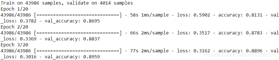

 
... ...

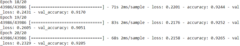
     the Fashion MNIST dataset only contained eight classes—for example, all the classes except for sandal and shirt. Someone built and trained a Keras model on that set and got reasonably good performance (>90% accuracy). Let’s call this model A

model_A.save("my_model_A.h5")

model_B = keras.models.Sequential()
model_B.add( keras.layers.Flatten(input_shape=[28,28]) )
for n_hidden in (300, 100, 50, 50, 50):
    model_B.add( keras.layers.Dense(n_hidden, activation="selu") )
    
model_B.add( keras.layers.Dense(1, activation="sigmoid") )

model_B.compile( loss="binary_crossentropy", 
                 optimizer=keras.optimizers.SGD(lr=1e-3),
                 metrics=['accuracy'])

history_B = model_B.fit( X_train_B, y_train_B, epochs=20,
                        validation_data=(X_valid_B, y_valid_B) )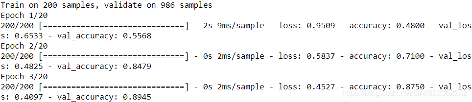

 
... ...

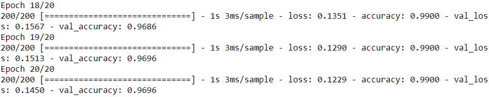
      You now want to tackle a different task: you have images of sandals and shirts, and you want to train a binary classifier (positive=shirt, negative=sandal). Your dataset is quite small; you only have 200 labeled images. When you train a new model for this task (let’s call it model B) with the same architecture as model A, it performs reasonably well (97% accuracy).

     First, you need to load model A and create a new model based on that model’s layers. 

     Let’s reuse all the layers except for the output layer:

model_A = keras.models.load_model("my_model_A.h5")
# reuse all the layers except for the output layer
model_B_on_A = keras.models.Sequential( model_A.layers[:-1] )
model_B_on_A.add( keras.layers.Dense(1, activation='sigmoid') )

     Note that model_A and model_B_on_A now share some layers. When you train model_B_on_A, it will also affect model_A. If you want to avoid that, you need to clone model_A before you reuse its layers. To do this, you clone model A’s architecture with clone_model(), then copy its weights (since clone_model() does not clone the weights):

model_A_clone = keras.models.clone_model( model_A )
model_A_clone.set_weights( model_A.get_weights() )

     Now you could train model_B_on_A for task B, but since the new output layer was initialized randomly it will make large errors (at least during the first few epochs), so there will be large error gradients that may wreck the reused weights. To avoid this, one approach is to freeze the reused layers during the first few epochs, giving the new layer some time to learn reasonable weights. To do this, set every layer’s trainable attribute to False and compile the model:

for layer in model_B_on_A.layers[:-1]:
    layer.trainable = False
    
model_B_on_A.compile( loss="binary_crossentropy",
                      optimizer=keras.optimizers.SGD(lr=1e-3),
                      metrics=['accuracy']
                    ) 

Note: You must always compile your model after you freeze or unfreeze layers.

     Now you can train the model for a few epochs, then unfreeze the reused layers (which requires compiling the model again) and continue training to fine-tune the reused layers for task B. After unfreezing the reused layers, it is usually a good idea to reduce the learning rate, once again to avoid damaging the reused weights:

history = model_B_on_A.fit( X_train_B, y_train_B, epochs=4,
                            validation_data=(X_valid_B, y_valid_B) )

for layer in model_B_on_A.layers[:-1]: #unfreeze
    layer.trainable=True
    
model_B_on_A.compile( loss="binary_crossentropy",
                      optimizer=keras.optimizers.SGD(lr=1e-3),
                      metrics=['accuracy']
                    )

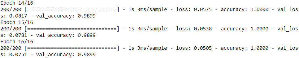
history = model_B_on_A.fit( X_train_B, y_train_B, epochs=16,
                            validation_data=(X_valid_B, y_valid_B) )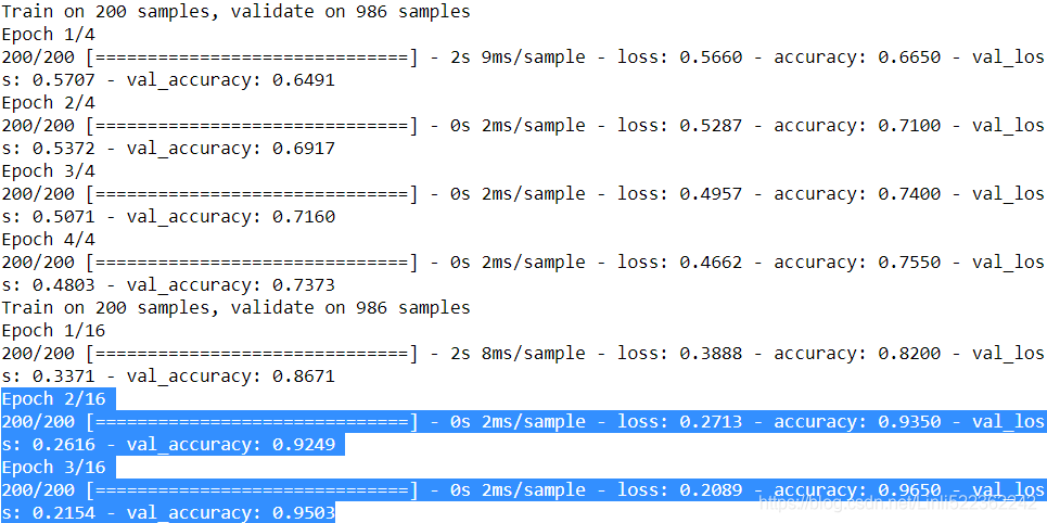

... ...

     So, what’s the final verdict?

model_B.evaluate(X_test_B, y_test_B)

 

model_B_on_A.evaluate(X_test_B, y_test_B)

 

     Well, this model’s test accuracy is 99.25%, which means that transfer learning reduced the error rate from 3.05%(1-0.9695) down to almost 0.75%(1-0.9925)! That’s a factor of four!

(1-0.9695) / (1-0.9925)

 

     Are you convinced? You shouldn’t be: I cheated! I tried many configurations until I found one that demonstrated a strong improvement. If you try to change the classes or the random seed, you will see that the improvement generally drops, or even vanishes or reverses. What I did is called “torturing the data until it confesses.交待” When a paper just looks too positive, you should be suspicious: perhaps the flashy new technique does not actually help much (in fact, it may even degrade performance), but the authors tried many variants and reported only the best results (which may be due to sheer luck), without mentioning how many failures they encountered on the way. Most of the time, this is not malicious at all, but it is part of the reason so many results in science can never be reproduced.

     Why did I cheat? It turns out that transfer learning does not work very well with small dense networks, presumably大概 because small networks learn few patterns, and dense networks learn very specific patterns, which are unlikely to be useful in other tasks. Transfer learning works best with deep convolutional neural networks, which tend to learn feature detectors that are much more general (especially in the lower layers). We will revisit transfer learning in Chapter 14, using the techniques we just discussed (and this time there will be no cheating, I promise!).

Unsupervised Pretraining无监督的预训练

     Suppose you want to tackle a complex task for which you don’t have much labeled training data, but unfortunately you cannot find a model trained on a similar task. Don’t lose hope! First, you should try to gather more labeled training data, but if you can’t, you may still be able to perform unsupervised pretraining (see Figure 11-5). Indeed, it is often cheap to gather unlabeled training examples, but expensive to label them. If you can gather plenty of unlabeled training data, you can try to use it to train an unsupervised model, such as an autoencoder or a generative adversarial对抗（性）的 network (see Chapter 17). Then you can reuse the lower layers of the autoencoder or the lower layers of the GAN’s discriminator鉴别器, add the output layer for your task on top, and finetune the final network using supervised learning (i.e., with the labeled training examples).

Boltzmann Machines#################

######################

3.14 Structured Probabilistic Models

     Machine learning algorithms often involve probability distributions over a very large number of random variables. Often, these probability distributions involve direct interactions between relatively few variables. Using a single function to describe the entire joint probability distribution can be very inefficient (both computationally and statistically).

     Instead of using a single function to represent a probability distribution, we can split a probability distribution into many factors that we multiply together.
     For example, suppose we have three random variables: a, b and c. Suppose that a influences the value of b and b influences the value of c, but that a and c are independent given b. We can represent the probability distribution over all three variables as a product of probability distributions over two variables:
(3.52)

     These factorizations因式分解 can greatly reduce the number of parameters needed to describe the distribution. Each factor uses a number of parameters that is exponential in the number of variables in the factor. This means that we can greatly reduce the cost of representing a distribution if we are able to find a factorization into distributions over fewer variables.

     We can describe these kinds of factorizations using graphs. Here we use the word “graph” in the sense of graph theory: a set of vertices that may be connected to each other with edges. When we represent the factorization因式分解 of a probability distribution with a graph当我们用图来表示概率分布的因式分解, we call it a structured probabilistic model结构化概率模型 or graphical model图模型.

     There are two main kinds of structured probabilistic models: directed and undirected. Both kinds of graphical models use a graph in which each node in the graph corresponds to a random variable, and an edge connecting two random variables means that the probability distribution is able to represent direct interactions between those two random variables.

     Directed models use graphs with directed edges, and they represent factorizations into conditional probability distributions它们代表分解为条件概率分布, as in the example above. Specifically, a directed model contains one factor for every random variable in the distribution, and that factor consists of the conditional distribution over given the parents of , denoted :
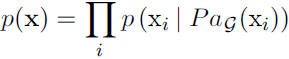(3.53)

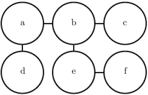
See figure 3.7 for an example of a directed graph and the factorization of probability distributions it represents.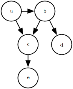
Figure 3.7: A directed graphical model over random variables a, b, c, d and e. This graph corresponds to probability distributions that can be factored as
 (3.54)
     This graph allows us to quickly see some properties of the distribution. For example, a and c interact directly, but a and e interact only indirectly via c.

 

     Undirected models use graphs with undirected edges, and they represent factorizations into a set of functions; unlike in the directed case, these functions are usually not probability distributions of any kind. Any set of nodes that are all connected to each other in is called a clique团. Each clique in an undirected model is associated with a factor . These factors are just functions, not probability distributions. The output of each factor must be non-negative, but there is no constraint that the factor must sum or integrate to 1 like a probability distribution.

     The probability of a configuration of random variables is proportional to the product of all of these factors—assignments that result in larger factor values are more likely. Of course, there is no guarantee that this product will sum to 1. We therefore divide by a normalizing constant Z, defined to be the sum or integral over all states of the product of the functions, in order to obtain a normalized probability distribution: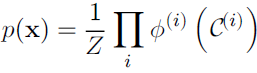
(3.55)

     See figure 3.8 for an example of an undirected graph and the factorization of probability distributions it represents.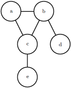
Figure 3.8: An undirected graphical model over random variables a, b, c, d and e. This graph corresponds to probability distributions that can be factored as
(3.56)

     This graph allows us to quickly see some properties of the distribution. For example, a and c interact directly, but a and e interact only indirectly via c.

     Keep in mind that these graphical representations of factorizations are a language for describing probability distributions. They are not mutually exclusive families of probability distributions. Being directed or undirected is not a property of a probability distribution; it is a property of a particular description of a probability distribution, but any probability distribution may be described in both ways.
######################

Cp16 Structured Probabilistic Models for Deep Learning

     A structured probabilistic model is a way of describing a probability distribution, using a graph to describe which random variables in the probability distribution interact with each other directly. Here we use “graph” in the graph theory sense—a set of vertices connected to one another by a set of edges. Because the structure of the model is defined by a graph, these models are often also referred to as graphical models.

     Structured probabilistic models use graphs (in the graph theory sense of “nodes” or “vertices” connected by edges) to represent interactions between random variables. Each node represents a random variable. Each edge represents a direct interaction. These direct interactions imply other, indirect interactions, but only the direct interactions need to be explicitly modeled.

     There is more than one way to describe the interactions in a probability distribution using a graph. In the following sections we describe some of the most popular and useful approaches. Graphical models can be largely divided into two categories: models based on directed acyclic[ˌeɪˈsaɪklɪk]无环的 graphs, and models based on undirected graphs.

16.2.1 Directed Models

     One kind of structured probabilistic model is the directed graphical model, otherwise known as the belief network or Bayesian network。

     Directed graphical models are called “directed” because their edges are directed, that is, they point from one vertex to another. This direction is represented in the drawing with an arrow. The direction of the arrow indicates which variable’s
probability distribution is defined in terms of the other’s. Drawing an arrow from a to b means that we define the probability distribution over b via a conditional distribution, with a as one of the variables on the right side of the conditioning bar. In other words, the distribution over b depends on the value of a.

     Continuing with the relay race接力赛跑 example from section 16.1, suppose we name Alice’s finishing time , Bob’s finishing time , and Carol’s finishing time . As we saw earlier, our estimate of depends on . Our estimate of depends directly on but only indirectly on . We can draw this relationship in a directed graphical model, illustrated in figure 16.2.

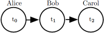Figure 16.2: A directed graphical model depicting the relay race example. Alice’s finishing time influences Bob’s finishing time , because Bob does not get to start running until Alice finishes. Likewise, Carol only gets to start running after Bob finishes, so Bob’s finishing time directly influences Carol’s finishing time .

     Formally, a directed graphical model defined on variables x is defined by a directed acyclic graph whose vertices are the random variables in the model, and a set of local conditional probability distributions where
gives the parents of in . The probability distribution over x is given by
 (16.1)

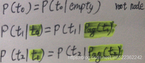
In our relay race example, this means that, using the graph drawn in figure 16.2,
  (16.2) ### Probability of occurrence of all variables

     This is our first time seeing a structured probabilistic model in action. We can examine the cost of using it, in order to observe how structured modeling has many advantages relative to unstructured modeling.

     Suppose we represented time by discretizing使离散 time ranging from minute 0 to minute 10 into 6 second chunks. This would make , and each be a discrete variable with 100 possible values(=60*10/6). If we attempted to represent p (, , ) with a table, it would need to store 999,999 values (100 values of × 100 values of ×100 values of , minus 1, since the probability of one of the configurations is made redundant多余 by the constraint that the sum of the probabilities be 1). 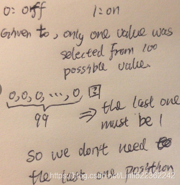If instead, we only make a table for each of the conditional probability distributions, then the distribution over requires 99 values, the table defining given requires 9900 values(=99×100,  100 since not given ), and so does the table defining given . This comes to a total of 19,899 values(99+99*100+99*100). This means that using the directed graphical model reduced our number of parameters by a factor of more than 50!

     In general, to model n discrete variables each having k values, the cost of the single table approach scales like , as we have observed before. Now suppose we build a directed graphical model over these variables. If m is the maximum number of variables appearing (on either side of the conditioning bar) in a single conditional probability distribution, then the cost of the tables for the directed model scales like . As long as we can design a model such that m << n, we get very dramatic savings.

     In other words, so long as each variable has few parents in the graph, the distribution can be represented with very few parameters. Some restrictions on the graph structure, such as requiring it to be a tree, can also guarantee that
operations like computing marginal or conditional distributions over subsets of variables are efficient.

     It is important to realize what kinds of information can and cannot be encoded in the graph. The graph encodes only simplifying assumptions about which variables are conditionally independent from each other. It is also possible to make other
kinds of simplifying assumptions. For example, suppose we assume Bob always runs the same regardless of how Alice performed. (In reality, Alice’s performance probably influences Bob’s performance—depending on Bob’s personality, if Alice runs especially fast in a given race, this might encourage Bob to push hard and match her exceptional performance, or it might make him overconfident and lazy). Then the only effect Alice has on Bob’s finishing time is that we must add Alice’s finishing time to the total amount of time we think Bob needs to run. This observation allows us to define a model with O(k ) parameters instead of . However, note that and are still directly dependent with this assumption, because represents the absolute time at which Bob finishes, not the total time he himself spends running. This means our graph must still contain an arrow from to . The assumption that Bob’s personal running time is independent from all other factors cannot be encoded in a graph over , , and . Instead, we encode this information in the definition of the conditional distribution itself. The conditional distribution is no longer a k ×k − 1 element table indexed by and but is now a slightly more complicated formula using only k − 1 parameters. The directed graphical model syntax does not place any constraint on how we define our conditional distributions. It only defines which variables they are allowed to
take in as arguments.

16.2.2 Undirected Models

     Directed graphical models give us one language for describing structured probabilistic models. Another popular language is that of undirected models, otherwise known as Markov random fields (MRFs) or Markov networks (Kindermann,
1980). As their name implies, undirected models use graphs whose edges are undirected.

     Directed models are most naturally applicable to situations where there is a clear reason to draw each arrow in one particular direction. Often these are situations where we understand the causality and the causality only flows in one direction. One such situation is the relay race example. Earlier runners affect the finishing times of later runners; later runners do not affect the finishing times of earlier runners.

     Not all situations we might want to model have such a clear direction to their interactions. When the interactions seem to have no intrinsic direction, or to operate in both directions, it may be more appropriate to use an undirected model.

     As an example of such a situation, suppose we want to model a distribution over three binary variables: whether or not you are sick, whether or not your coworker is sick, and whether or not your roommate is sick. As in the relay race example, we can make simplifying assumptions about the kinds of interactions that take place. Assuming that your coworker and your roommate do not know each other, it is very unlikely that one of them will give the other an infection such as a cold directly. This event can be seen as so rare that it is acceptable not to model it. However, it is reasonably likely that either of them could give you a cold, and that you could pass it on to the other. We can model the indirect transmission of a cold from your coworker to your roommate by modeling the transmission of the cold from your coworker to you and the transmission of the cold from you to your
roommate.

     In this case, it is just as easy for you to cause your roommate to get sick as it is for your roommate to make you sick, so there is not a clean, uni-directional narrative on which to base the model. This motivates using an undirected model. As with directed models, if two nodes in an undirected model are connected by an edge, then the random variables corresponding to those nodes interact with each other directly. Unlike directed models, the edge in an undirected model has no arrow, and is not associated with a conditional probability distribution.

     We denote the random variable representing your health as , the random variable representing your roommate’s health as , and the random variable representing your colleague’s health as . See figure 16.3 for a drawing of the graph representing this scenario.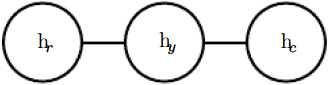
Figure 16.3: An undirected graph representing how your roommate’s health , your health , and your work colleague’s health affect each other. You and your roommate might infect each other with a cold, and you and your work colleague might do the same, but assuming that your roommate and your colleague do not know each other, they can only infect each other indirectly via you.

     Formally, an undirected graphical model is a structured probabilistic model defined on an undirected graph . For each clique团  in the graph, a factor (also called a clique potential团势能) measures the affinity密切关系 of the variables in that clique for being in each of their possible joint states. The factors are constrained to be non-negative. Together they define an unnormalized probability distribution
(16.3)

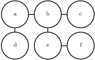
     The unnormalized probability distribution is efficient to work with so long as all the cliques are small. It encodes the idea that states with higher affinity are more likely. However, unlike in a Bayesian network, there is little structure to the definition of the cliques, so there is nothing to guarantee that multiplying them together will yield a valid probability distribution. See figure 16.4 for an example of reading factorization information from an undirected graph.

Figure 16.4: This graph implies that p(a, b, c, d, e, f) can be written as  for an appropriate choice of the functions.

     Our example of the cold spreading between you, your roommate, and your colleague contains two cliques.One clique contains and . The factor for this clique can be defined by a table, and might have values resembling these: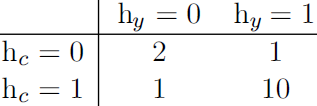

     A state of 1 indicates good health, while a state of 0 indicates poor health (having been infected with a cold). Both of you are usually healthy, so the corresponding state has the highest affinity. The state where only one of you is
sick has the lowest affinity, because this is a rare state. The state where both of you are sick (because one of you has infected the other) is a higher affinity state, though still not as common as the state where both are healthy.

To complete the model, we would need to also define a similar factor for the clique containing and .

16.2.3 The Partition Function

     While the unnormalized未归一化 probability distribution is guaranteed to be non-negative everywhere, it is not guaranteed to sum or integrate to 1. To obtain a valid probability distribution, we must use the corresponding normalized probability distribution:
(16.4)          

where Z is the value that results in the probability distribution summing or integrating to 1:
(16.5)

     You can think of Z as a constant when the functions are held constant. Note that if the functions have parameters, then Z is a function of those parameters. It is common in the literature to write Z with its arguments omitted to save space.
The normalizing constant Z is known as the partition function, a term borrowed from statistical physics.

     Since Z is an integral or sum over all possible joint assignments of the state x it is often intractable难对付的 to compute. In order to be able to obtain the normalized probability distribution of an undirected model, the model structure and the definitions of the functions must be conducive to computing Z efficiently. In the context of deep learning, Z is usually intractable. Due to the intractability of computing Z exactly, we must resort to approximations. Such approximate algorithms are the topic of chapter 18.

     One important consideration to keep in mind when designing undirected models is that it is possible to specify the factors in such a way that Z does not exist. This happens if some of the variables in the model are continuous and the integral of over their domain diverges. For example, suppose we want to model a single scalar variable x ∈ with a single clique potential = . In this case,    
(16.6)

     Since this integral diverges, there is no probability distribution corresponding to this choice of . Sometimes the choice of some parameter of the functions determines whether the probability distribution is defined. For example, for
, the β parameter determines whether Z exists. Positive β results in a Gaussian distribution over x but all other values of β make impossible to normalize.

     One key difference between directed modeling and undirected modeling is that directed models are defined directly in terms of probability distributions from the start, while undirected models are defined more loosely by functions that are then converted into probability distributions. This changes the intuitions one must develop in order to work with these models. One key idea to keep in mind while working with undirected models is that the domain of each of the variables
has dramatic effect on the kind of probability distribution that a given set of functions corresponds to. For example, consider an n-dimensional vector-valued random variable x and an undirected model parametrized by a vector of biases b. Suppose we have one clique for each element of x, . What kind of probability distribution does this result in? The answer is that we do not have enough information, because we have not yet specified the domain of x.

• If x ∈ , then the integral defining Z diverges ###and ### and no probability distribution exists.
• If x ∈ , then p(x) factorizes into n independent distributions, with .
• If the domain of x is the set of elementary basis vectors ({[1, 0, . . . , 0], [0, 1, . . . ,0], . . . , [0, 0, . . . , 1]} ) then p(x) = softmax(b), so a large value of actually reduces for .

Often, it is possible to leverage the effect of a carefully chosen domain of a variable in order to obtain complicated
behavior from a relatively simple set of functions. We will explore a practical application of this idea later, in section 20.6.

16.2.4 Energy-Based Models

     Many interesting theoretical results about undirected models depend on the assumption that ∀x, > 0. A convenient way to enforce this condition is to use an energy-based model (EBM) where  (16.7)
and E(x) is known as the energy function. Because exp(z ) is positive for all z, this guarantees that no energy function will result in a probability of zero for any state x. Being completely free to choose the energy function makes learning simpler. If we learned the clique potentials directly, we would need to use constrained optimization to arbitrarily impose some specific minimal probability value. By learning the energy function, we can use unconstrained optimization.The probabilities in an energy-based model can approach arbitrarily close to zero but never reach it.

     Any distribution of the form given by equation 16.7 is an example of a Boltzmann distribution. For this reason, many energy-based models are called Boltzmann machines (Fahlman et al., 1983; Ackley et al., 1985; Hinton et al., 1984; Hinton and Sejnowski, 1986). There is no accepted guideline for when to call a model an energy-based model and when to call it a Boltzmann machine. The term Boltzmann machine was first introduced to describe a model with exclusively binary variables, but today many models such as the mean-covariance restricted Boltzmann machine incorporate real-valued variables as well. While Boltzmann machines were originally defined to encompass both models with and without latent variables, the term Boltzmann machine is today most often used to designate models with latent variables, while Boltzmann machines without latent variables are more often called Markov random fields or log-linear models.

     Cliques in an undirected graph correspond to factors of the unnormalized probability function. Because exp(a) exp(b) = exp( a+ b ), this means that different cliques in the undirected graph correspond to the different terms of the energy function. In other words, an energy-based model is just a special kind of Markov network: the exponentiation makes each term in the energy function correspond to a factor for a different clique. See figure 16.5 for an example of how to read the form of the energy function from an undirected graph structure. One can view an energy-based model with multiple terms in its energy function as being a product of experts (Hinton, 1999). Each term in the energy function corresponds to another factor in the probability distribution. Each term of the energy function can be thought of as an “expert” that determines whether a particular soft constraint is satisfied. Each expert may enforce only one constraint that concerns only a low-dimensional projection of the random variables, but when combined by multiplication of probabilities, the experts together enforce a complicated high dimensional constraint.

     Figure 16.5: This graph implies that E(a, b, c, d, e, f) can be written as + for an appropriate choice of the per-clique energy functions. Note that we can obtain the functions in figure 16.4 by setting each  to the exponential of the corresponding negative energy, e.g., .

     One part of the definition of an energy-based model serves no functional purpose from a machine learning point of view: the − sign in equation 16.7. This − sign could be incorporated into the definition of E. For many choices of the function E, the learning algorithm is free to determine the sign of the energy anyway. The − sign is present primarily to preserve compatibility between the machine learning literature and the physics literature.

     Many algorithms that operate on probabilistic models do not need to compute but only . For energy-based models with latent variables h, these algorithms are sometimes phrased in terms of the negative of this quantity, called the free energy: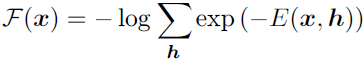
(16.8)

16.7.1 Example: The Restricted Boltzmann Machine

     The restricted Boltzmann machine (RBM) (Smolensky, 1986) or harmonium is the quintessential example of how graphical models are used for deep learning. The RBM is not itself a deep model. Instead, it has a single layer of latent variables
that may be used to learn a representation for the input. In chapter 20, we will see how RBMs can be used to build many deeper models. Here, we show how the RBM exemplifies举例说明 many of the practices used in a wide variety of deep graphical models: its units are organized into large groups called layers, the connectivity between layers is described by a matrix, the connectivity is relatively dense, the model is designed to allow efficient Gibbs sampling, and the emphasis of the model design is on freeing the training algorithm to learn latent潜 variables whose semantics were not specified by the designer. Later, in section 20.2, we will revisit the RBM in more detail.

     The canonical典范 RBM is an energy-based model with binary visible and hidden units. Its energy function is 
(16.10)
where b, c , and W are unconstrained, real-valued, learnable parameters. We can see that the model is divided into two groups of units: v and h, and the interaction between them is described by a matrix W . The model is depicted graphically
in figure 16.14. As this figure makes clear, an important aspect of this model is that there are no direct interactions between any two visible units or between any two hidden units (hence the “restricted,” a general Boltzmann machine may have arbitrary connections).

Figure 16.14: An RBM drawn as a Markov network

The restrictions on the RBM structure yield the nice properties (16.11)

and (16.12)

The individual conditionals are simple to compute as well. For the binary RBM we obtain: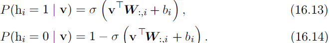

     Together these properties allow for efficient block Gibbs sampling, which alternates between sampling all of h simultaneously and sampling all of v simultaneously. Samples generated by Gibbs sampling from an RBM model are shown in
figure 16.15.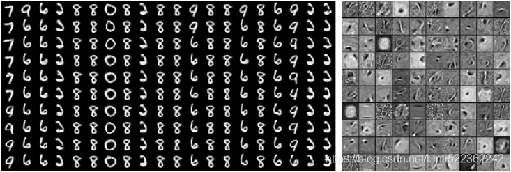

     Figure 16.15: Samples from a trained RBM, and its weights. Image reproduced with permission from LISA (2008). (Left)Samples from a model trained on MNIST, drawn using Gibbs sampling. Each column is a separate Gibbs sampling process. Each row represents the output of another 1,000 steps of Gibbs sampling. Successive连续 samples are highly correlated with one another. (Right)The corresponding weight vectors. Compare this to the samples and weights of a linear factor model, shown in figure 13.2. The samples here are much better because the RBM prior p(h) is not constrained to be factorial. The RBM can learn which features should appear together when sampling. On the other hand, the RBM posterior p(h | v) is factorial, while the sparse coding posterior p(h | v) is not, so the sparse coding model may be better for feature extraction. Other models are able to have both a non-factorial p(h) and a non-factorial p(h | v).
###

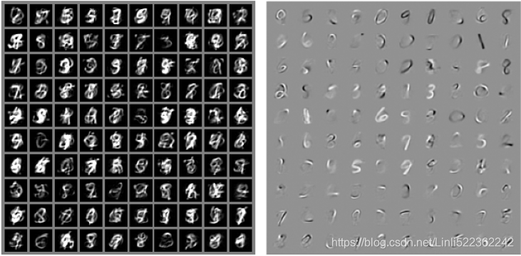
     Figure 13.2: Example samples and weights from a spike and slab sparse coding model trained on the MNIST dataset. (Left)The samples from the model do not resemble类似 the training examples. At first glance, one might assume the model is poorly fit. (Right)The weight vectors of the model have learned to represent penstrokes笔划 and sometimes complete digits. The model has thus learned useful features. The problem is that the factorial prior over features results in random subsets of features being combined. Few such subsets are appropriate to form a recognizable MNIST digit. This motivates the development of generative models that have more powerful distributions over their latent codes. Figure reproduced with permission from Goodfellow et al. (2013d).

###

     Since the energy function(16.10) itself is just a linear function of the parameters, it is easy to take its derivatives. For example,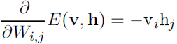
(16.15)

These two properties—efficient Gibbs sampling and efficient derivatives—make training convenient.

     Training the model induces a representation h of the data v. We can often use  as a set of features to describe v.

     Overall, the RBM demonstrates the typical deep learning approach to graphical models: representation learning accomplished via layers of latent variables, combined with efficient interactions between layers parametrized by matrices.

Chapter 20 Deep Generative Models

20.1 Boltzmann Machines

     We define the Boltzmann machine over a d-dimensional binary random vector x ∈ . The Boltzmann machine is an energy-based model (section 16.2.4 ), meaning we define the joint probability distribution using an energy function:
    (20.1) <== 

where E (x) is the energy function and Z is the partition function that ensures that  = 1. The energy function of the Boltzmann machine is given by
  (20.2)

where U is the “weight” matrix of model parameters and b is the vector of bias parameters.

     In the general setting of the Boltzmann machine, we are given a set of training examples, each of which are n-dimensional. Equation 20.1 describes the joint probability distribution over the observed variables. While this scenario is certainly
viable, it does limit the kinds of interactions between the observed variables to those described by the weight matrix. Specifically, it means that the probability of one unit being on is given by a linear model (logistic regression) from the values of
the other units.

     The Boltzmann machine becomes more powerful when not all the variables are observed. In this case, the latent variables, can act similarly to hidden units in a multi-layer perceptron and model higher-order interactions among the visible units. Just as the addition of hidden units to convert logistic regression into an MLP results in the MLP being a universal approximator of functions, a Boltzmann machine with hidden units is no longer limited to modeling linear relationships between variables. Instead, the Boltzmann machine becomes a universal approximator of probability mass functions over discrete variables (Le Roux and Bengio, 2008).

     Formally, we decompose the units x into two subsets: the visible units v and the latent (or hidden) units h. The energy function becomes  (20.3)

Boltzmann Machine Learning Learning algorithms for Boltzmann machines are usually based on maximum likelihood. All Boltzmann machines have an intractable partition function, so the maximum likelihood gradient must be approximated
using the techniques described in chapter 18

20.2 Restricted Boltzmann Machines

     Invented under the name harmonium (Smolensky, 1986), restricted Boltzmann machines are some of the most common building blocks of deep probabilistic models. We have briefly described RBMs previously, in section 16.7.1. Here we review the
previous information and go into more detail. RBMs are undirected probabilistic graphical models containing a layer of observable variables and a single layer of latent variables. RBMs may be stacked (one on top of the other) to form deeper
models. See figure 20.1 for some examples. In particular, figure 20.1a shows the graph structure of the RBM itself. It is a bipartite graph, with no connections permitted between any variables in the observed layer or between any units in the
latent layer.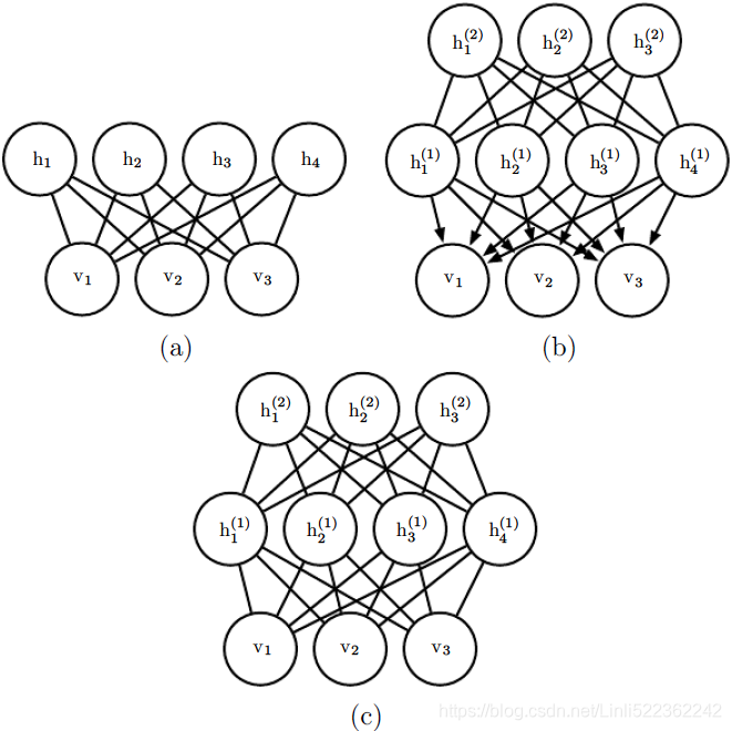
Figure 20.1: Examples of models that may be built with restricted Boltzmann machines. (a)The restricted Boltzmann machine itself is an undirected graphical model based on
a bipartite graph, with visible units in one part of the graph and hidden units in the other part. There are no connections among the visible units, nor any connections among the hidden units. Typically every visible unit is connected to every hidden unit but it is possible to construct sparsely connected RBMs such as convolutional RBMs. (b)A deep belief network is a hybrid graphical model involving both directed and undirected connections. Like an RBM, it has no intralayer connections. However, a DBN has multiple hidden layers, and thus there are connections between hidden units that are in separate layers. All of the local conditional probability distributions needed by the deep belief network are copied directly from the local conditional probability distributions of its constituent RBMs. Alternatively, we could also represent the deep belief network with
a completely undirected graph, but it would need intralayer connections to capture the dependencies between parents. (c)A deep Boltzmann machine is an undirected graphical model with several layers of latent variables. Like RBMs and DBNs, DBMs lack intralayer connections. DBMs are less closely tied to RBMs than DBNs are. When initializing a DBM from a stack of RBMs, it is necessary to modify the RBM parameters slightly. Some kinds of DBMs may be trained without first training a set of RBMs.

     We begin with the binary version of the restricted Boltzmann machine, but as we see later there are extensions to other types of visible and hidden units.

     More formally, let the observed layer consist of a set of binary random variables which we refer to collectively with the vector v. We refer to the latent or hidden layer of binary random variables as h.

     Like the general Boltzmann machine, the restricted Boltzmann machine is an energy-based model with the joint probability distribution specified by its energy function: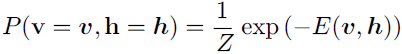
(20.4)        <==

The energy function for an RBM is given by

  (20.5) <==         

and Z is the normalizing constant known or sum == 1 as the partition function

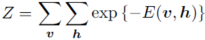(20.6)  

    It is apparent from the definition of the partition function Z that the naive method of computing Z (exhaustively summing over all states) could be computationally intractable, unless a cleverly designed algorithm could exploit regularities in the probability distribution to compute Z faster. In the case of restricted Boltzmann machines, Long and Servedio (2010) formally proved that the partition function Z is intractable. The intractable partition function Z implies that the normalized joint probability distribution P(v) is also intractable to evaluate.

######################

     Boltzmann machines were invented in 1985 by Geoffrey Hinton and Terrence Sejnowski. Just like Hopfield nets, they are fully connected ANNs, but they are based on stochastic neurons: instead of using a deterministic step function to decide what value to output, these neurons output 1 with some probability, and 0 otherwise. The probability function that these ANNs use is based on the Boltzmann distribution (used in statistical mechanics) hence their name. Equation E-1 gives the probability that a particular neuron will output a 1.

Equation E-1. Probability that the neuron will output 1
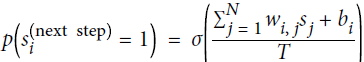<==and 

• is the neuron’s state (0 or 1).
• is the connection weight between the and neurons. Note that = 0.
• is the neuron’s bias term. We can implement this term by adding a bias neuron to the network.
• N is the number of neurons in the network.
• T is a number called the network’s temperature; the higher the temperature, the more random the output is (i.e., the more the probability approaches 50%).
• σ is the logistic function. logistic sigmoid activation function

     Neurons in Boltzmann machines are separated into two groups: visible units and hidden units (see Figure E-2). All neurons work in the same stochastic way, but the visible units are the ones that receive the inputs and from which outputs are read.

Figure E-2. Boltzmann machine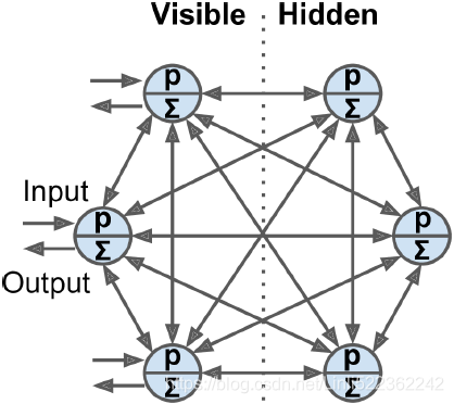

     Because of its stochastic nature, a Boltzmann machine will never stabilize使稳定 into a fixed configuration; instead, it will keep switching between many configurations. If it is left running for a sufficiently long time, the probability of observing a particular configuration will only be a function of the connection weights and bias terms, not of the original configuration (similarly, after you shuffle a deck of cards一副纸牌 for long enough, the configuration of the deck does not depend on the initial state). When the network reaches this state where the original configuration is “forgotten,” it is said to be in thermal equilibrium热平衡 (although its configuration keeps changing all the time). By setting the network parameters appropriately, letting the network reach thermal equilibrium, and then observing its state, we can simulate a wide range of probability distributions. This is called a generative model生成模型.

     Training a Boltzmann machine means finding the parameters that will make the network approximate the training set’s probability distribution. For example, if there are three visible neurons and the training set contains 75% (0, 1, 1) triplets, 10% (0, 0, 1) triplets, and 15% (1, 1, 1) triplets, then after training a Boltzmann machine, you could use it to generate random binary triplets with about the same probability distribution. For example, about 75% of the time it would output the (0, 1, 1) triplet.

     Such a generative model can be used in a variety of ways. For example, if it is trained on images, and you provide an incomplete or noisy image to the network, it will automatically “repair” the image in a reasonable way. You can also use a generative model for classification. Just add a few visible neurons to encode the training image’s class (e.g., add 10 visible neurons and turn on only the fifth neuron when the training image represents a 5). Then, when given a new image, the network will automatically turn on the appropriate visible neurons, indicating the image’s class (e.g., it will turn on the fifth visible neuron if the image represents a 5).

     Unfortunately, there is no efficient technique to train Boltzmann machines. However, fairly efficient algorithms have been developed to train restricted Boltzmann machines(RBMs).

Restricted Boltzmann Machines受限制的

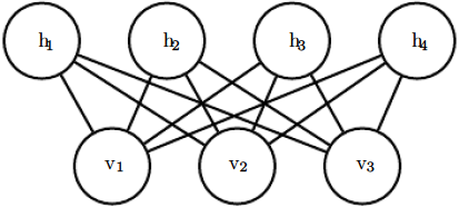
     An RBM is simply a Boltzmann machine in which there are no connections between visible units or between hidden units, only between visible and hidden units. For example, Figure E-3 represents an RBM with three visible units and four hidden
units.
Figure E-3. Restricted Boltzmann machine                               Figure E-2. Boltzmann machine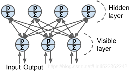
                  
     A very efficient training algorithm called Contrastive Divergence was introduced in 2005 by Miguel Á. Carreira-Perpiñán and Geoffrey Hinton. Here is how it works: for each training instance x, the algorithm starts by feeding it to the network by setting
the state of the visible units to . Then you compute the state of the hidden units by applying the stochastic equation described before (Equation E-1 ). This gives you a hidden vector h (where is equal to the state of the unit). Next you compute the state of the visible units, by applying the same stochastic equation. This gives you a vector xʹ. Then once again you compute the state of the hidden units, which gives you a vector hʹ. Now you can update each connection weight by applying the rule in Equation E-2, where η is the learning rate.

Equation E-2. Contrastive divergence weight update

     The great benefit of this algorithm is that it does not require waiting for the network to reach thermal equilibrium: it just goes forward, backward, and forward again, and that’s it. This makes it incomparably more efficient than previous algorithms, and it
was a key ingredient to the first success of Deep Learning based on multiple stacked RBMs.

#################

Unsupervised Pretraining无监督的预训练

     Suppose you want to tackle a complex task for which you don’t have much labeled training data, but unfortunately you cannot find a model trained on a similar task. Don’t lose hope! First, you should try to gather more labeled training data, but if you can’t, you may still be able to perform unsupervised pretraining (see Figure 11-5). Indeed, it is often cheap to gather unlabeled training examples, but expensive to label them. If you can gather plenty of unlabeled training data, you can try to use it to train an unsupervised model, such as an autoencoder or a generative adversarial对抗（性）的 network (see Chapter 17). Then you can reuse the lower layers of the autoencoder or the lower layers of the GAN’s discriminator鉴别器, add the output layer for your task on top, and finetune the final network using supervised learning (i.e., with the labeled training examples).
Figure 11-5. In unsupervised training, a model is trained on the unlabeled data (or on all the data) using an unsupervised learning technique, then it is fine-tuned for the final task on the labeled data using a supervised learning technique; the unsupervised part may train one layer at a time as shown here, or it may train the full model directly

     It is this technique that Geoffrey Hinton and his team used in 2006 and which led to the revival of neural networks and the success of Deep Learning. Until 2010, unsupervised pretraining—typically with restricted Boltzmann machines (RBMs; see Appendix E)—was the norm for deep nets, and only after the vanishing gradients problem was alleviated did it become much more common to train DNNs purely using supervised learning. Unsupervised pretraining (today typically using autoencoders or GANs(generative adversarial networks) rather than RBMs) is still a good option when you have a complex task to solve, no similar model you can reuse, and little labeled training data but plenty of unlabeled training data.

     Note that in the early days of Deep Learning it was difficult to train deep models, so people would use a technique called greedy layer-wise pretraining贪婪分层预训练 (depicted in Figure 11-5). They would first train an unsupervised model with a single layer, typically an RBM, then they would freeze that layer and add another one on top of it, then train the model again (effectively just training the new layer), then freeze the new layer and add another layer on top of it, train the model again, and so on( Finally, it is fine-tuned for the final task on the labeled data using a supervised learning technique). Nowadays, things are much simpler: people generally train the full unsupervised model in one shot (i.e., in Figure 11-5, just start directly at step three) and use autoencoders or GANs rather than RBMs.

Pretraining on an Auxiliary[ɔːɡˈzɪliəri]辅助的 Task

     If you do not have much labeled training data, one last option is to train a first neural network on an auxiliary task for which you can easily obtain or generate labeled training data, then reuse the lower layers of that network for your actual task. The first neural network’s lower layers will learn feature detectors that will likely be reusable by the second neural network.

     For example, if you want to build a system to recognize faces, you may only have a few pictures of each individual—clearly not enough to train a good classifier. Gathering hundreds of pictures of each person would not be practical. You could, however,
gather a lot of pictures of random people on the web and train a first neural network to detect whether or not two different pictures feature the same person. Such a network would learn good feature detectors for faces, so reusing its lower layers would allow you to train a good face classifier that uses little training data.

     For natural language processing (NLP) applications, you can download a corpus语料库 of millions of text documents and automatically generate labeled data from it. For example, you could randomly mask out some words and train a model to predict what the missing words are (e.g., it should predict that the missing word in the sentence “What ___ you saying?” is probably “are” or “were”). If you can train a model to reach good performance on this task, then it will already know quite a lot about language, and you can certainly reuse it for your actual task and fine-tune it on your labeled data (we will discuss more pretraining tasks in Chapter 15).

     Self-supervised learning is when you automatically generate the labels from the data itself(typically using a
heuristic[hjʊˈrɪstɪk]启发式的 algorithm), then you train a model on the resulting “labeled” dataset using supervised learning techniques. Since this approach requires no human labeling whatsoever无论怎样, it is best classified as a form of unsupervised learning.

Faster Optimizers

     Training a very large deep neural network can be painfully slow. So far we have seen four ways to speed up training (and reach a better solution):

• applying a good initialization strategy for the connection weights, # such as truncated_normal( shape, mean=0.0, stdev=1.0 ) # range: [ mean-2*stddev, mean+2*stddev ]
• using a good activation function,
• using Batch Normalization,
• and reusing parts of a pretrained network (possibly built on an auxiliary task or using unsupervised learning).

Another huge speed boost comes from using a faster optimizer than the regular Gradient Descent optimizer. In this section we will present the most popular algorithms: momentum optimization, Nesterov Accelerated Gradient, AdaGrad, RMSProp, and finally Adam and Nadam optimization.

Momentum Optimization http://www.cs.toronto.edu/~hinton/absps/momentum.pdf

     Imagine a bowling ball rolling down a gentle slope on a smooth surface: it will start out slowly, but it will quickly pick up momentum until it eventually reaches terminal velocity (if there is some friction or air resistance). This is the very simple idea behind momentum optimization, proposed by Boris Polyak in 1964.13 In contrast, regular Gradient Descent will simply take small, regular steps down the slope, so the algorithm will take much more time to reach the bottom.

     Recall that Gradient Descent updates the weights θ by directly subtracting the gradient of the cost function J(θ) with regard to the weights () multiplied by the learning rate η. The equation is: θ ← θ – OR https://blog.csdn.net/Linli522362242/article/details/104005906. It does not care about what the earlier gradients were. If the local gradient is tiny, it goes very slowly.
############################################################

http://www.cs.toronto.edu/~hinton/absps/momentum.pdf

Equation 11-4. Momentum algorithm

1.  # it subtracts the local gradient * η from the momentum vector m, m is negative
2.              #  it updates the weights by adding this momentum vector m,  note m is negative

     Momentum optimization cares a great deal about what previous gradients were: at each iteration, it subtracts the local gradient from the momentum vector m (multiplied by the learning rate η), and it updates the weights by adding this momentum
vector (see Equation 11-4). In other words, the gradient is used for acceleration, not for speed. To simulate some sort of friction摩擦 mechanism and prevent the momentum m from growing too large, the algorithm introduces a new hyperparameter β, called the momentum, which must be set between 0 (high friction) and 1 (no friction). A typical momentum value is 0.9.

     You can easily verify that if the gradient remains constant, the terminal velocity (i.e., the maximum size of the weight updates) is equal to that gradient multiplied by the learning rate η multiplied by 1/(1–β) (ignoring the sign).

In keras:

The update rule for θ with gradient g when momentum(β) is 0.0:

The update rule when momentum is larger than 0.0(β>0): is negative since ,有方向gradent是向下（negative）,但是在计算机计算过程为了好处理使用了正值

if nesterov is False, gradient is evaluated at . if nesterov is True, gradient is evaluated at , and the variables always store θ+mv instead of theta

Equation 11-5. Nesterov Accelerated Gradient algorithm

•  m is negative since ,
• 

############################################################

Equation 11-4. Momentum algorithm

1. #adds the local gradient * η to the momentum vector m, note m is positive
2.    #it updates the weights by simply subtracting this momentum vector m,  note m is positive

特点：

• 下降初期时，使用上一次参数更新，下降方向一致，乘上较大的β能够进行很好的加速
• 下降中后期时，在局部最小值来回震荡的时候，-->0，β使得更新幅度增大，跳出陷阱
• 在梯度改变方向的时候(梯度上升，梯度方向与βm相反)，能够减少更新总而言之，momentum项能够在相关方向加速SGD，抑制振荡，从而加快收敛

     Momentum optimization cares a great deal about what previous gradients were: at each iteration, it adds the local gradient to the momentum vector m (multiplied by the learning rate η), and it updates the weights by simply subtracting this momentum vector (see Equation 11-4). In other words, the gradient is used for acceleration, not for speed. To simulate some sort of friction摩擦 mechanism and prevent the momentum from growing too large, the algorithm introduces a new hyperparameter β, called the momentum, which must be set between 0 (high friction) and 1 (no friction). A typical momentum value is 0.9.

     You can easily verify that if the gradient remains constant, the terminal velocity (i.e., the maximum size of the weight updates, ###Here is m###) is equal to that gradient multiplied by the learning rate η multiplied by 1/(1–β)       
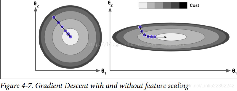
For example, if β = 0.9, then the terminal velocity is equal to 10 times the gradient times the learning rate, so momentum optimization ends up going 10 times faster than Gradient Descent! This allows momentum optimization to escape from plateaus停滞时期 much faster than Gradient Descent. We saw in Chapter 4 that when the inputs have very different scales, the cost
function will look like an elongated bowl (see Figure 4-7). Gradient Descent goes down the steep slope陡坡 quite fast, but then it takes a very long time to go down the valley深谷. In contrast, momentum optimization will roll down the valley faster and faster
until it reaches the bottom (the optimum). In deep neural networks that don’t use Batch Normalization, the upper layers will often end up having inputs with very different scales, so using momentum optimization helps a lot. It can also help roll past local optima.

     Due to the momentum, the optimizer may overshoot超调 a bit, then come back, overshoot again, and oscillate[ˈɑsɪleɪt]使振荡 like this many times before stabilizing at the minimum. This is one of the reasons it’s good to have a bit of friction in the system: it gets rid of these oscillations and thus speeds up convergence.

     Implementing momentum optimization in Keras is a no-brainer: just use the SGD optimizer and set its momentum hyperparameter, then lie back and profit!

optimizer = keras.optimizers.SGD(lr=0.001, momentum=0.9)

     The one drawback of momentum optimization is that it adds yet another hyperparameter to tune. However, the momentum value of 0.9 usually works well in practice and almost always goes faster than regular Gradient Descent.
https://zhuanlan.zhihu.com/p/77380412

class MomentumGradientDescent(MiniBatchGradientDescent):
    def __init__(self, gamma=0.9, **kwargs):
        self.gamma = gamma  # gammar also called momentum, 当gamma=0时，相当于小批量随机梯度下降
        super(MomentumGradientDescent, self).__init__(**kwargs)

    def fit(self, X, y):
        X = np.c_[np.ones(len(X)), X]
        n_samples, n_features = X.shape

        self.theta = np.ones(n_features)
        self.velocity = np.zeros_like(self.theta) ################
        self.loss_ = [0]

        self.i = 0
        while self.i < self.n_iter:#n_iter: epochs
            self.i += 1
            if self.shuffle:
                X, y = self._shuffle(X, y)

            errors = []
            for j in range(0, n_samples, self.batch_size):
                mini_X, mini_y = X[j: j + self.batch_size], y[j: j + self.batch_size]
                error = mini_X.dot(self.theta) - mini_y
                errors.append(error.dot(error))
                mini_gradient = 1/ self.batch_size * mini_X.T.dot(error)# without*2 since cost/loss
                self.velocity = self.velocity * self.gamma + self.eta * mini_gradient
                self.theta -= self.velocity
                                                      #loss*1/2 for convenient computing gradient    
            loss = 1 / (2 * self.batch_size) * np.mean(errors)
            delta_loss = loss - self.loss_[-1] #当结果改善的变动低于某个阈值时，程序提前终止
            self.loss_.append(loss)
            if np.abs(delta_loss) < self.tolerance:
                break
        return self

Nesterov Accelerated Gradient

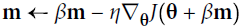
     One small variant to momentum optimization, proposed by Yurii Nesterov in 1983,14 is almost always faster than vanilla momentum optimization. The Nesterov Accelerated Gradient (NAG) method, also known as Nesterov momentum optimization, measures the gradient of the cost function not at the local position θ but slightly ahead in the direction of the momentum, at θ + βm (see Equation 11-5).

Equation 11-5. Nesterov Accelerated Gradient algorithm

• 
• 

     This small tweak works because in general the momentum vector m will be pointing in the right direction (i.e., toward the optimum), so it will be slightly more accurate to use the gradient measured a bit farther in that direction rather than using the gradient at the original position, as you can see in Figure 11-6 (where represents the gradient of the cost function measured at the starting point θ, and represents the gradient at the point located at θ + βm, Note: θ*βm<0).    

Figure 11-6. Regular versus Nesterov Momentum optimization(==β);  the former applies the gradients computed before the momentum step(βm), while the latter applies the gradients###### computed after.

     As you can see, the Nesterov update ends up slightly closer to the optimum. After a while, these small improvements add up and NAG ends up being significantly faster than regular Momentum optimization. Moreover, note that when the momentum pushes the weights across a valley, continues to push further across the valley, while  pushes back toward the bottom of the valley（更正方向）. This helps reduce oscillations and thus converges faster.

     NAG（Nesterov Accelerated Gradient） is generally faster than regular momentum optimization. To use it, simply set nesterov=True when creating the SGD optimizer:

optimizer = keras.optimizers.SGD(lr=0.001, momentum=0.9, nesterov=True)

 

class NesterovAccelerateGradient(MomentumGradientDescent):
    def __init__(self, **kwargs):
        super(NesterovAccelerateGradient, self).__init__(**kwargs)

    def fit(self, X, y):
        X = np.c_[np.ones(len(X)), X]
        n_samples, n_features = X.shape #n_features: n_features+1

        #OR random_uniform(shape=[n_features,1],minval=-1.0, maxval=1.0,)
        self.theta = np.ones(n_features)   
        self.velocity = np.zeros_like(self.theta)#################
        self.loss_ = [0]

        self.i = 0
        while self.i < self.n_iter:
            self.i += 1
            if self.shuffle:
                X, y = self._shuffle(X, y)

            errors = []
            for j in range(0, n_samples, self.batch_size):
                mini_X, mini_y = X[j: j + self.batch_size], y[j: j + self.batch_size]
                # gamma also called momentum
                error = mini_X.dot(self.theta - self.gamma * self.velocity) - mini_y############  
                errors.append(error.dot(error))
                mini_gradient = 1 / self.batch_size * mini_X.T.dot(error)
                self.velocity = self.velocity * self.gamma + self.eta * mini_gradient
                self.theta -= self.velocity
            loss = 1 / (2 * self.batch_size) * np.mean(errors)
            delta_loss = loss - self.loss_[-1]
            self.loss_.append(loss)
            if np.abs(delta_loss) < self.tolerance:
                break
        return self

AdaGrad

     Consider the elongated bowl problem again: Gradient Descent starts by quickly going down the steepest slope, which does not point straight toward the global optimum, then it very slowly goes down to the bottom of the valley. It would be nice if the algorithm could correct its direction earlier to point a bit more toward the global optimum. The AdaGrad algorithm achieves this correction by scaling down the gradient vector along the steepest dimensions (see Equation 11-6).

Equation 11-6. AdaGrad algorithm

1.          # accumulates s 约束项regularizer: 1/
2. 

特点：

• 前期accumulates较小的时候， regularizer较大，能够放大梯度
• 后期accumulates较大的时候，regularizer较小，能够约束梯度
• 适合处理稀疏梯度

缺点：

• 由公式可以看出，仍依赖于人工设置一个全局学习率
• learning rate设置过大的话，会使regularizer过于敏感，对梯度的调节太大
• 中后期，分母上梯度平方的累加将会越来越大，使-->0,使gradent-->0，使得训练提前结束

     The first step accumulates the square of the gradients into the vector s (recall that the ⊗ symbol represents the element-wise multiplication). This vectorized form is equivalent to computing for each element of the vector s; in other words, each accumulates the squares of the partial derivative of the cost function with regard to parameter . If the cost function is steep along the dimension, then
will get larger and larger at each iteration.

     The second step is almost identical to Gradient Descent, but with one big difference: the gradient vector is scaled down by a factor of s + ε (the ⊘ symbol represents the element-wise division, and ε is a smoothing term to avoid division by zero, typically set to ). This vectorized form is equivalent to simultaneously computing  for all parameters .

     In short, this algorithm decays the learning rate, but it does so faster for steep dimensions than for dimensions with gentler slopes. This is called an adaptive learning rate. It helps point the resulting updates more directly toward the global optimum (see Figure 11-7). One additional benefit is that it requires much less tuning of the learning rate hyperparameter η.

Figure 11-7. AdaGrad versus Gradient Descent: the former can correct its direction earlier to point to the optimum

     AdaGrad frequently performs well for simple quadratic problems, but it often stops too early when training neural networks. The learning rate gets scaled down so much that the algorithm ends up stopping entirely before reaching the global optimum. So even though Keras has an Adagrad optimizer, you should not use it to train deep neural networks (it may be efficient for simpler tasks such as Linear Regression, though). Still, understanding AdaGrad is helpful to grasp the other adaptive learning rate optimizers.

class AdaptiveGradientDescent(MiniBatchGradientDescent):
    def __init__(self, epsilon=1e-6, **kwargs):
        self.epsilon = epsilon
        super(AdaptiveGradientDescent, self).__init__(**kwargs)

    def fit(self, X, y):
        X = np.c_[np.ones(len(X)), X]
        n_samples, n_features = X.shape
        self.theta = np.ones(n_features)
        self.loss_ = [0]

        gradient_sum = np.zeros(n_features)##############s

        self.i = 0
        while self.i < self.n_iter:
            self.i += 1
            if self.shuffle:
                X, y = self._shuffle(X, y)

            errors = []
            for j in range(0, n_samples, self.batch_size):
                mini_X, mini_y = X[j: j + self.batch_size], y[j: j + self.batch_size]
                error = mini_X.dot(self.theta) - mini_y  
                errors.append(error.dot(error))
                mini_gradient = 1 / self.batch_size * mini_X.T.dot(error)  
                gradient_sum += mini_gradient ** 2 ##############
                adj_gradient = mini_gradient / (np.sqrt(gradient_sum + self.epsilon))
                self.theta -= self.eta * adj_gradient
            loss = 1 / (2 * self.batch_size) * np.mean(errors)

            delta_loss = loss - self.loss_[-1]
            self.loss_.append(loss)
            if np.abs(delta_loss) < self.tolerance:
                break
        return self

RMSProp(RootMeanSquareProp)

     As we’ve seen, AdaGrad runs the risk of slowing down a bit too fast and never converging to the global optimum. The RMSProp algorithm fixes this by accumulating only the gradients from the most recent iterations (as opposed to all the gradients since the beginning of training). It does so by using exponential decay in the first step (see Equation 11-7).

Equation 11-7. RMSProp algorithm

1. 
2. 

     The decay rate β is typically set to 0.9. Yes, it is once again a new hyperparameter, but this default value often works well, so you may not need to tune it at all.

As you might expect, Keras has an RMSprop optimizer:

optimizer = keras.optimizers.RMSprop(lr=0.001, rho=0.9)

     Note that the rho argument corresponds to β in Equation 11-7. Except on very simple problems, this optimizer almost always performs much better than AdaGrad. In fact, it was the preferred optimization algorithm of many researchers until Adam optimization came around.

class RMSProp(MiniBatchGradientDescent):
    def __init__(self, gamma=0.9, epsilon=1e-6, **kwargs):
        self.gamma = gamma #called momenturm B
        self.epsilon = epsilon
        super(RMSProp, self).__init__(**kwargs)

    def fit(self, X, y):
        X = np.c_[np.ones(len(X)), X]
        n_samples, n_features = X.shape
        self.theta = np.ones(n_features)
        self.loss_ = [0]

        gradient_exp = np.zeros(n_features)

        self.i = 0
        while self.i < self.n_iter:
            self.i += 1
            if self.shuffle:
                X, y = self._shuffle(X, y)

            errors = []
            for j in range(0, n_samples, self.batch_size):
                mini_X, mini_y = X[j: j + self.batch_size], y[j: j + self.batch_size]
                error = mini_X.dot(self.theta) - mini_y
                errors.append(error.dot(error))
                mini_gradient = 1 / self.batch_size * mini_X.T.dot(error)
                ###################################################
                gradient_exp = self.gamma * gradient_exp + (1 - self.gamma) * mini_gradient**2
                gradient_rms = np.sqrt(gradient_exp + self.epsilon)
                self.theta -= self.eta / gradient_rms * mini_gradient

            loss = 1 / (2 * self.batch_size) * np.mean(errors)
            delta_loss = loss - self.loss_[-1]
            self.loss_.append(loss)
            if np.abs(delta_loss) < self.tolerance:
                break
        return self

Adam and Nadam Optimization
https://blog.csdn.net/Linli522362242/article/details/107086444