


This chapter covers
- A first example of a neural network
- Tensors and tensor operations
- How neural networks learn via backpropagation and gradient descent
Understanding deep learning requires familiarity with many simple mathematical concepts: tensors, tensor operations, differentiation, gradient descent, and so on. Our goal in this chapter will be to build your intuition about these notions without getting overly technical. In particular, we’ll steer away from避开 mathematical notation, which can be off-putting令人不愉快的;老是推托的 for those without any mathematics background and isn’t strictly necessary to explain things well.
To add some context for tensors and gradient descent, we’ll begin the chapter with a practical example of a neural network. Then we’ll go over every new concept that’s been introduced, point by point. Keep in mind that these concepts will be essential for you to understand the practical examples that will come in the following chapters!
After reading this chapter, you’ll have an intuitive understanding of how neural networks work, and you’ll be able to move on to practical applications—which will start with chapter 3https://blog.csdn.net/Linli522362242/article/details/106433059.
2.1 A first look at a neural network
Let’s look at a concrete example of a neural network that uses the Python library Keras to learn to classify handwritten digits. Unless you already have experience with Keras or similar libraries, you won’t understand everything about this first example right away. You probably haven’t even installed Keras yet; that’s fine. In the next chapter, we’ll review each element in the example and explain them in detail. So don’t worry if some steps seem arbitrary or look like magic to you! We’ve got to start somewhere.
The problem we’re trying to solve here is to classify grayscale images of handwritten digits (28 × 28 pixels) into their 10 categories (0 through 9). We’ll use the MNIST dataset, a classic in the machine-learning community, which has been around almost as long as the field itself and has been intensively studied. It’s a set of 60,000 training images, plus 10,000 test images, assembled by the National Institute of Standards and Technology (the NIST in MNIST ) in the 1980s. You can think of “solving” MNIST as the “Hello World” of deep learning—it’s what you do to verify that your algorithms are working as expected. As you become a machine-learning practitioner, you’ll see
MNIST come up over and over again, in scientific papers, blog posts, and so on. You can see some MNIST samples in figure 2.1. Figure 2.1 MNIST sample digits
Note on classes and labels
- In machine learning, a category in a classification problem is called a class. Data points are called samples. The class associated with a specific sample is called a label.
You don’t need to try to reproduce this example on your machine just now. If you wish to, you’ll first need to set up Keras, which is covered in section 3.3https://blog.csdn.net/Linli522362242/article/details/106537459.
import tensorflow as tf
from tensorflow import keras

tf.__version__ ![]()
keras.__version__
The MNIST dataset comes preloaded in Keras, in the form of a set of four Numpy arrays.
Loading the MNIST dataset in Keras
- The MNIST dataset is publicly available at MNIST handwritten digit database, Yann LeCun, Corinna Cortes and Chris Burges and consists of the following four parts:
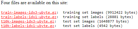
Test dataset images: t10k-images-idx3-ubyte.gz (1.6 MB, 7.8 MB unzipped, and 10,000 examples)
Test dataset labels: t10k-labels-idx1-ubyte.gz (5 KB, 10 KB unzipped, and 10,000 labels)
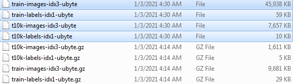
After downloading the files, simply run the next code cell to unzip the files.import sys import gzip import shutil import os parent_dir = os.getcwd() # C:\Users\liqin\0deepLearningWithPython path = os.path.join(parent_dir, 'mnist') os.mkdir(path) # os.getcwd() 'C:\\Users\\liqin\\0deepLearningWithPython' os.chdir(path) # os.getcwd() # 'C:\\Users\\liqin\\0deepLearningWithPython\\mnist' # sys.version_info # sys.version_info(major=3, minor=7, micro=4, releaselevel='final', serial=0) # print(sys.version_info > (3, 0)) # 判断python是否为3.0以上(包括3.0)# True # print(sys.version_info > (3, 7, 0)) # 判断python是否为3.7.0以上(包括3.7.0)# True # print(sys.version_info > (3, 7, 4)) # 判断python是否为3.7.6以上(包括3.7.6)# True # print(sys.version_info > (3, 7, 7)) # 判断python是否为3.7.7以上(包括3.7.7)# False # if major > 3 if ( sys.version_info >(3,0) ): writemode='wb' else: writemode='w' zipped_mnist = [f for f in os.listdir() if f.endswith('ubyte.gz')] for z in zipped_mnist: # filename: exclude '.gz' with gzip.GzipFile(z, mode='rb') as decompressed, open(z[:-3], writemode) as outfile: outfile.write( decompressed.read() )
MNIST handwritten digit database, Yann LeCun, Corinna Cortes and Chris Burges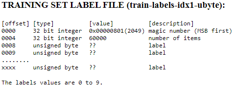

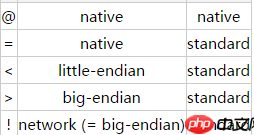
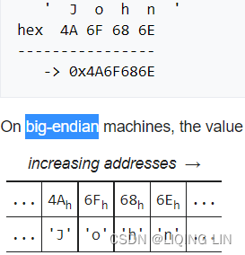
• >: This is big-endian—it defines the order in which a sequence of bytes is stored; if you are unfamiliar with the terms big-endian and littleendian, you can find an excellent article about Endianness on Wikipedia: https://en.wikipedia.org/wiki/Endianness
 and
and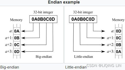
 vs
vs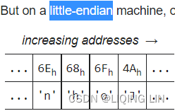
import os
import struct
import numpy as np

def load_mnist( path, kind='train' ):
    """Load Mnist data from 'path'"""
    labels_path = os.path.join( path,
                                '%s-labels-idx1-ubyte' % kind)
    images_path = os.path.join( path,
                                '%s-images-idx3-ubyte' % kind)

    with open(labels_path, 'rb') as lbpath:
        # the magic number : a description of the file protocol from the file buffer
        # n: the number of items (n) from the file buffer
        # >: This is big-endian—it defines the order in which a sequence of bytes is stored
        # https://docs.python.org/3/library/struct.html
        # I: This is an unsigned integer, 1 (standard size) = 4 bytes
        #          struct.unpack(format, buffer)
        # first 32 bits = 4 bytes
        # first two 32 bits = 4 bytes + 4bytes = II to represent magic number and number of items
        magic, n = struct.unpack( '>II', # II: required 2 unsigned integers
                                  lbpath.read(8) # 8 = 4*2
                                )
        # print(magic, n) # 2049(==0x00000801,
                          #          00:The first 2 bytes are always 0.
                          #          0000: a magic number;       #0D:float(4 bytes); 0E:double(8 bytes)
                          #              08(0x08): unsigned byte; 09:signed byte; 0C:int(4 bytes)
                          #                01: vector) 01 for vectors, 02 for matrices..
                          # 60000(vector)
        # OR 2049 60000
        # after lbpath.read(8), unpack data start: labels
        # numpy.fromfile(file, dtype=float, count=- 1, sep='', offset=0, *, like=None)
        #                Construct an array from data in a text or binary file.
        labels = np.fromfile( lbpath,
                              dtype=np.uint8 # Data type of the returned array
                            )

    with open(images_path, 'rb') as imgpath:
        # first four 32 bits = 4 bytes + 4bytes + bytes + 4bytes = IIII
        magic, num, rows, cols = struct.unpack( ">IIII", # IIII: required 4 unsigned integers
                                                imgpath.read(16) # 16=4*4
                                              )
        # print(magic, num, rows, cols) # 2051(0x00000803==,
                                        #        00:The first 2 bytes are always 0.
                                        #        0000 is a magic number;
                                        #            08(0x08):unsigned byte; 0B:short(2 bytes)
                                        #              03: 3D )
                                        # 60000
                                        # 28 28 (3D)
        # OR 2051 60000 28 28
        # after lbpath.read(16), unpack data start: pixeles
        images = np.fromfile( imgpath,
                              dtype=np.uint8 # Data type of the returned array
                            ).reshape( len(labels), 784 ) #784=28*28 #np.uint8,也就是0~255
                    # before .reshape(), shape=len(labels)*28*28
        images = ( (images/255.)-.5 )*2 # /(255*255)
    return images, labels

X_train, y_train = load_mnist(path,
                              kind='train')
print('Rows: %d, columns: %d' % (X_train.shape[0], X_train.shape[1]) )

X_test, y_test = load_mnist(r'C:\Users\liqin\0deepLearningWithPython\mnist',
                            kind='t10k')
print( 'Rows: %d, columns: %d' % (X_test.shape[0], X_test.shape[1]) )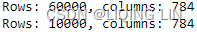
-
import tensorflow_datasets as tfds

mnist, mnist_info = tfds.load('mnist', with_info=True,
                               shuffle_files=False)
print( mnist_info )
cp13_2_PNN Training_tfrecord files_image process_mnist_gradient_iris_exponent_Adagrad_Adam_tanh_Relu_LIQING LIN的博客-CSDN博客
 -
import tensorflow_datasets as tfds

# 0. Fetch the `tfds.core.DatasetBuilder` by name:
mnist_bldr = tfds.builder('mnist')
# 1. Create the tfrecord files (no-op if already exists)
#    Generate the data (when `download=True`):
mnist_bldr.download_and_prepare()
# shuffle_files=False : This prevented initial shuffling
#                      if the initial shuffling was not turned off,
#                      it would incur reshuffling of the dataset every time
#                      we fetched a mini-batch of data.
# An example of this behavior:
# the number of labels in the validation datasets changes
#      due to reshuffling of the train/validation splits.
# This can cause false performance estimation of the model,
#      since the train/validation datasets are indeed mixed
# Control whether to shuffle the files between each epoch
#       (TFDS store big datasets in multiple smaller files).

# as_supervised : Default False
# if True, the returned tf.data.Dataset will have a "2-tuple structure" (input, label)
#          according to builder.info.supervised_keys.
# If False, the default, the returned tf.data.Dataset will have a "dictionary"
#           with all the features.
# 2. Load the `tf.data.Dataset` object:
datasets = mnist_bldr.as_dataset( shuffle_files=False )# Load data from disk as tf.data.Datasets

print( datasets.keys() ) # ==> dict_keys([Split('train'), Split('test')])

mnist_train_orig, mnist_test_orig = \
    datasets['train'], datasets['test'] #'PrefetchDataset' object

mnist_train = mnist_train_orig.map(
    lambda item: (tf.cast(item['image'], tf.float32)/255.0,
                  tf.cast(item['label'], tf.int32)))

mnist_test = mnist_test_orig.map(
    lambda item: (tf.cast(item['image'], tf.float32)/255.0,
                  tf.cast(item['label'], tf.int32)))

tf.random.set_seed(1)
BUFFER_SIZE = 10000
BATCH_SIZE = 64

mnist_train = mnist_train.shuffle(buffer_size=BUFFER_SIZE,
                                  reshuffle_each_iteration=False
                                 )# ==> preprocess_map ==> batch
# mnist_valid and mnist_train are from same train.tfrecord files
mnist_valid = mnist_train.take(100)#.batch(BATCH_SIZE)
mnist_train = mnist_train.skip(100)#.batch(BATCH_SIZE)

from collections import Counter

def count_labels(ds):
    counter = Counter()
    for example in ds:
        counter.update([example[1].numpy()])
    return counter

print( 'Count of labels:', count_labels(mnist_valid) )
print( 'Count of labels:', count_labels(mnist_valid) )

#print("minist_train\n")
#for example in mnist_train.take(10):
#    print( "label:",example[1], ", shape:",example[0].shape )
#print("minist_valid\n")
#for example in mnist_valid.take(10):
#    print( "label:",example[1], ", shape:",example[0].shape )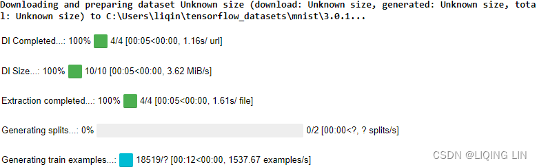
...

OR
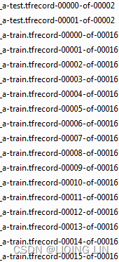
Because the data is relatively small, it only needs to be stored in 2 tfrecord files, which causes the shuffle_files=True in the following code to not work, and the output result is the same as the previous one. However, if there is a lot of data, it will be divided into multiple tfrecord files, and shuffle_files=True will work.# 0. Fetch the `tfds.core.DatasetBuilder` by name: mnist_bldr = tfds.builder('mnist') # 1. Create the tfrecord files (no-op if already exists) # Generate the data (when `download=True`): mnist_bldr.download_and_prepare() # as_supervised : Default False # if True, the returned tf.data.Dataset will have a "2-tuple structure" (input, label) # according to builder.info.supervised_keys. # If False, the default, the returned tf.data.Dataset will have a "dictionary" # with all the features. # Control whether to shuffle the files between each epoch # (TFDS store big datasets in multiple smaller files). # 2. Load the `tf.data.Dataset` object: datasets = mnist_bldr.as_dataset( shuffle_files=True, as_supervised=True )# Load data from disk as tf.data.Datasets # print( datasets.keys() ) # ==> dict_keys([Split('train'), Split('test')]) mnist_train_orig, mnist_test_orig = \ datasets['train'], datasets['test'] #'PrefetchDataset' object mnist_train = mnist_train_orig.map( lambda image, label: (tf.cast(image, tf.float32)/255.0, tf.cast(label, tf.int32) )) mnist_test = mnist_test_orig.map( lambda image, label: (tf.cast(image, tf.float32)/255.0, tf.cast(label, tf.int32) )) tf.random.set_seed(1) BUFFER_SIZE = 10000 BATCH_SIZE = 64 mnist_train = mnist_train.shuffle(buffer_size=BUFFER_SIZE, reshuffle_each_iteration=False )# ==> preprocess_map ==> batch # mnist_valid and mnist_train are from same train.tfrecord files mnist_valid = mnist_train.take(100)#.batch(BATCH_SIZE) mnist_train = mnist_train.skip(100)#.batch(BATCH_SIZE) from collections import Counter def count_labels(ds): counter = Counter() for image, label in ds: counter.update([label.numpy()]) return counter print('Count of labels:', count_labels(mnist_valid)) print('Count of labels:', count_labels(mnist_valid)) print("minist_train") for image, label in mnist_train.take(10): print( "label:",label, ", shape:", image.shape ) print("mnist_valid") for image, label in mnist_valid.take(10): print( "label:",label, ", shape:", image.shape )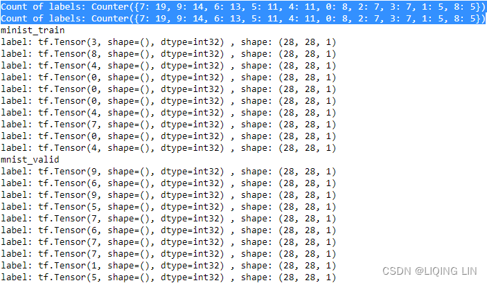
Because the data is relatively small, it only needs to be stored in 2 tfrecord files, which causes the shuffle_files=True in the following code to not work, and the output result is the same as the previous one. However, if there is a lot of data, it will be divided into multiple tfrecord files, and shuffle_files=True will work.
But,
 https://blog.csdn.net/Linli522362242/article/details/112386820
Let's simulate the result
print('Count of labels:', count_labels(mnist_valid))
# shuffle_files=True, change the 'order' of tfrecord files
# the tfrecord file we take data will be different with shuffle_files=False
mnist_valid = mnist_train.take(100)#.batch(BATCH_SIZE)
mnist_train = mnist_train.skip(100)#.batch(BATCH_SIZE)

from collections import Counter

def count_labels(ds):
    counter = Counter()
    for image, label in ds:
        counter.update([label.numpy()])
    return counter

print('Count of labels:', count_labels(mnist_valid))
- tf.keras.datasets.mnist.load_data
@keras_export("keras.datasets.mnist.load_data")
def load_data(path="mnist.npz"):
    """Loads the MNIST dataset.
    This is a dataset of 60,000 28x28 grayscale images of the 10 digits,
    along with a test set of 10,000 images.
    More info can be found at the
    [MNIST homepage](http://yann.lecun.com/exdb/mnist/).
    Args:
      path: path where to cache the dataset locally
        (relative to `~/.keras/datasets`).
    Returns:
      Tuple of NumPy arrays: `(x_train, y_train), (x_test, y_test)`.
    **x_train**: uint8 NumPy array of grayscale image data with shapes
      `(60000, 28, 28)`, containing the training data. Pixel values range
      from 0 to 255.
    **y_train**: uint8 NumPy array of digit labels (integers in range 0-9)
      with shape `(60000,)` for the training data.
    **x_test**: uint8 NumPy array of grayscale image data with shapes
      (10000, 28, 28), containing the test data. Pixel values range
      from 0 to 255.
    **y_test**: uint8 NumPy array of digit labels (integers in range 0-9)
      with shape `(10000,)` for the test data.
    Example:
    ```python
    (x_train, y_train), (x_test, y_test) = keras.datasets.mnist.load_data()
    assert x_train.shape == (60000, 28, 28)
    assert x_test.shape == (10000, 28, 28)
    assert y_train.shape == (60000,)
    assert y_test.shape == (10000,)
    ```
    License:
      Yann LeCun and Corinna Cortes hold the copyright of MNIST dataset,
      which is a derivative work from original NIST datasets.
      MNIST dataset is made available under the terms of the
      [Creative Commons Attribution-Share Alike 3.0 license.](
      https://creativecommons.org/licenses/by-sa/3.0/)
    """
    origin_folder = (
        "https://storage.googleapis.com/tensorflow/tf-keras-datasets/"
    )
    path = get_file(
        path,
        origin=origin_folder + "mnist.npz",
        file_hash="731c5ac602752760c8e48fbffcf8c3b850d9dc2a2aedcf2cc48468fc17b673d1",  # noqa: E501
    )
    with np.load(path, allow_pickle=True) as f:
        x_train, y_train = f["x_train"], f["y_train"]
        x_test, y_test = f["x_test"], f["y_test"]

        return (x_train, y_train), (x_test, y_test)
from keras.datasets import mnist
# from tensorflow import keras
                                          # keras.datasets.mnist.load_data()
(train_images, train_labels), (test_images, test_labels) = mnist.load_data()- train_images and train_labels form the training set, the data that the model will learn from.
- The model will then be tested on the test set, test_images and test_labels.
- The images are encoded as Numpy arrays, and the labels are an array of digits, ranging from 0 to 9.
- The images and labels have a one-to-one correspondence.

Let’s look at the training data:
print( train_images.shape, test_images.shape )
print( len(train_labels),  len(test_labels) )

train_labels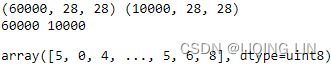
test_labels ![]()
The workflow will be as follows:
- First, we’ll feed the neural network the training data, train_images and train_labels .
- The network will then learn to associate images and labels.
- Finally, we’ll ask the network to produce predictions for test_images , and we’ll verify whether these predictions match the labels from test_labels
Let’s build the network
from keras import models
from keras import layers

network = models.Sequential()
network.add( layers.Dense( 512,
                           activation='relu',
                           input_shape=(28*28,)
                           use_bias=True,                       # default
                           bias_initializer='zeros',            # default
                           kernel_initializer='glorot_uniform', # default
                         )
           )
network.add( layers.Dense( 10, activation='softmax') )
The core building block of neural networks is the layer, a data-processing module that you can think of as a filter for data. Some data goes in, and it comes out in a more useful form. Specifically, layers extract representations out of the data fed into them—hopefully, representations that are more meaningful for the problem at hand. Most of deep learning consists of chaining together simple layers that will implement a form of progressive data distillation数据蒸馏. A deep-learning model is like a sieve/ sɪv /筛子,滤网 for data processing, made of a succession/ səkˈseʃ(ə)n /连续不断的人(物) of increasingly refined data filters—the layers.
###############################
https://www.tensorflow.org/api_docs/python/tf/keras/initializers
Each neuron can be initialized with specifc weights via the kernel_initializer parameter. There are a few choices, the most common of which are listed as follows:
- • random_uniform : Weights are initialized to uniformly random small values in the range -0.05 to 0.05.
tf.keras.initializers.RandomUniform(
    minval=-0.05, maxval=0.05, seed=None
)
Initializer that generates tensors with a uniform distribution.
- • random_normal : Weights are initialized according to a Gaussian distribution, with zero mean and a small standard deviation of 0.05. For those of you who are not familiar with Gaussian distribution, think about a symmetric "bell curve" shape.
tf.keras.initializers.RandomNormal(
    mean=0.0, stddev=0.05, seed=None
)
Initializer that generates tensors with a normal distribution.
- • zero : All weights are initialized to zero. (Initializer that generates tensors initialized to 0.)
- We need the signal to flow properly in both directions: in the forward direction when making predictions, and in the reverse direction when backpropagating gradients. We don’t want the signal to die out消失, nor do we want it to explode and saturate. For the signal to flow properly, the authors argue that
we need the variance of the outputs of each layer to be equal to the variance of its inputs,
and we also need the gradients to have equal variance before and after flowing through a layer in the reverse direction (please check out the paper if you are interested in the mathematical details).
It is actually not possible to guarantee both unless the layer has an equal number of input and output connections, but they proposed a good compromise妥协 that has proven to work very well in practice: the connection weights must be initialized randomly as described in Equation 11-1('glorot_uniform' OR 'glorot_normal'), whereand
are the number of input and output connections for the layer whose weights are being initialized (also called fan-in and fan-out;
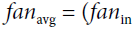
 ). This initialization strategy is often called Xavier initialization (after the author’s first name), or sometimes Glorot initialization.
https://blog.csdn.net/Linli522362242/article/details/106935910
The general idea behind Xavier initialization is to roughly balance the variance of the gradients across different layers大致平衡不同层之间的梯度变化. Otherwise, some layers may get too much attention during training while the other layers lag behind落后.
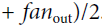
https://blog.csdn.net/Linli522362242/article/details/113710166 - 'glorot_uniform': uniform distribution between ‐r and +r,
with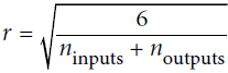 OR
OR OR
OR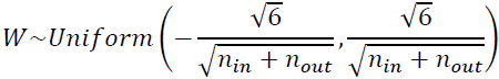
- 'glorot_normal' : Normal(Gaussian) distribution with mean 0 and standard deviation
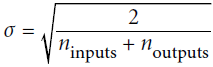 OR
OR 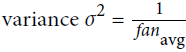
- 'HeNormal': It draws samples from a truncated normal distribution centered on 0 with
fan_inis the number of input units in the weight tensor. - 'HeUniform': Draws samples from a uniform distribution within
[-limit, limit], wherefan_inis the number of input units in the weight tensor). - 'LecunNormal': Draws samples from a truncated normal distribution centered on 0 with
fan_inis the number of input units in the weight tensor.
LeCun initialization is equivalent to Glorot initialization when
- 'LecunUniform':Draws samples from a uniform distribution within
[-limit, limit], wherefan_inis the number of input units in the weight tensor).
LeCun initialization is equivalent to Glorot initialization when - Table 11-1. Initialization parameters for each type of activation function


###############################
Here, our network consists of a sequence of two Dense layers, which are densely connected (also called fully connected) neural layers. The second (and last) layer is a 10-way softmax layer, which means it will return an array of 10 probability scores (summing to 1). Each score will be the probability that the current digit image belongs to one of our 10 digit classes.
To make the network ready for training, we need to pick three more things, as part of the compilation step:
- A loss function('objective function')—How the network will be able to measure its performance on the training data, and thus how it will be able to steer/ stɪr /引导 itself in the right direction.
which is used by the optimizer to navigate the space of weights (frequently, objective functions are called either loss functions or cost functions and the process of optimization is defined as a process of loss minimization
The loss is the quantity you’ll attempt to minimize during training, so it should represent a measure of success for the task you’re trying to solve - An optimizer—The mechanism through which the network will update itself based on the data it sees and its loss function.
which is the specifc algorithm used to update weights while we train our model
The optimizer specifies the exact way in which the gradient of the loss will be used to update parameters: for instance, it could be the RMSP rop optimizer, SGD with momentum, and so on. - Metrics to monitor during training and testing—Here, we’ll only care about accuracy (the fraction of the images that were correctly classified).
we need to evaluate the trained model.
The exact purpose of the loss function and the optimizer will be made clear through-out the next two chapters.
VVVVVVVVVVVVVVVVVVVVVVVVVVV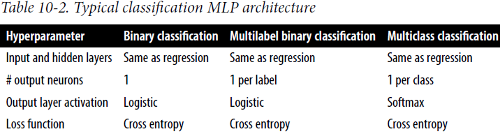
 https://blog.csdn.net/Linli522362242/article/details/108414534
- Equation 4-19. Softmax score for class k :
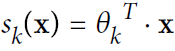
Note that each class has its own dedicated parameter vector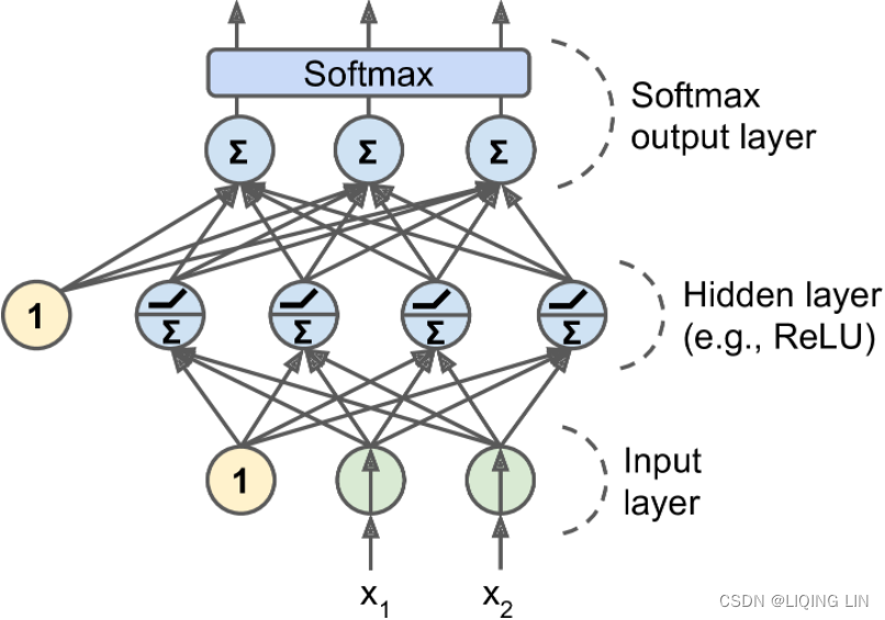
- Equation 4-20. Softmax function
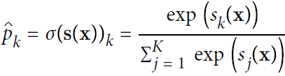
Softmax function takes an K-dimensional vector of real numbers and transforms it into a vector of real number in range (0,1) which add up to 1.
This property of softmax function that it outputs a probability distribution makes it suitable for probabilistic interpretation in classification tasks.
K is the number of classes(output units or neurons)
s(x) is a vector containing the scores of each class for the instance x.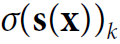 is the estimated probability that the instance x belongs to class k given the scores of each class for that instance.
 -
Derivative of Softmax
From quotient rule we know that for, we have
-
If, Differentiate
contained in the numerator and denominator
If, Differentiate
in the denominator
So the derivative of the softmax function is given as,
Or using Kronecker delta:
-
- Equation 4-21. Softmax Regression classifier prediction

<==argmax - Equation 4-22 Cross entropy cost function
Minimize: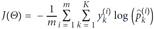
 is equal to 1 if the target class for the
 th instance is
; otherwise, it is equal to 0.
Notice that when there are just two classes (K = 2), this cost function is equivalent to the Logistic Regression’s cost function (log loss; see Equation 4-17
-
Derivative of Cross Entropy Loss:
for each sample
for, K is the number of classes (on the output layer)
From derivative of softmax we derived earlier,
for
all inputs=>softmax func=>argmax =>
output(the probility
of the
class)
argmax =>output(the probility
of the
class)
- Equation 4-23. Cross entropy gradient vector for class k
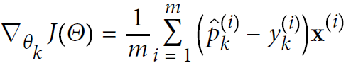 <==
<==and
Note that each class has its own dedicated parameter vector
Now you can compute the gradient vector for every class, then use Gradient Descent (or any other optimization algorithm) to find the parameter matrixthat minimizes the cost function.
RMSprop (Root Mean Square propagation) :
As we’ve seen, AdaGrad runs the risk of slowing down a bit too fast and never converging to the global optimum. The RMSProp algorithm fixes this by accumulating only the gradients from the most recent iterations (as opposed to all the gradients since the beginning of training). It does so by using exponential decay in the first step (see Equation 11-7).
OR RMSprop as well divides the learning rate by an exponentially decaying average of squared gradients.
Equation 11-7. RMSProp algorithm OR
OR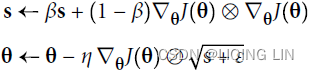
The decay rate β (or )is typically set to 0.9. Yes, it is once again a new hyperparameter, but this default value often works well, so you may not need to tune it at all. while a good default value for the learning rate η is 0.001.
# to denote the gradient at time step
in tensor:tensorflow/rmsprop.py at master · tensorflow/tensorflow · GitHub
"""One-line documentation for rmsprop module.
rmsprop algorithm [tieleman2012rmsprop]
A detailed description of rmsprop.
- maintain a moving (discounted) average of the square of gradients
- divide gradient by the root of this average

mean_square = decay * mean_square{t-1} + (1-decay) * gradient ** 2
# momentum Defaults to 0.0.
mom = momentum * mom{t-1} + learning_rate * g_t /
        sqrt(mean_square + epsilon)
delta = - mom
This implementation of RMSProp uses plain momentum, not Nesterov momentum.
The centered version additionally maintains a moving (discounted) average of the
gradients, and uses that average to estimate the variance:
################
mean_grad = decay * mean_grad{t-1} + (1-decay) * gradient
################
mean_square = decay * mean_square{t-1} + (1-decay) * gradient ** 2
mom = momentum * mom{t-1} + learning_rate * g_t /
        sqrt(mean_square - mean_grad**2 + epsilon)
                           ############
delta = - mom
"""
in kera:keras/rmsprop.py at v2.10.0 · keras-team/keras · GitHub
centered : Boolean. If True, gradients are normalized by the estimated variance of the gradient通过梯度的估计方差对梯度进行归一化;
if False, by the uncentered second moment.
OR
Setting this to True may help with training, but is slightly more expensive in terms of computation and memory. Defaults to False.
            ######224
            # mean_square: at iteration t, the mean of ( all gradients in mini-batch )
            # mean_square = decay * mean_square{t-1} + (1-decay) * gradient ** 2
            rms_t = coefficients["rho"] * rms
                    + coefficients["one_minus_rho"] * tf.square(grad)
            # tf.compat.v1.assign( ref, value, v
                                   alidate_shape=None, use_locking=None, name=None )
            # return : A Tensor that will hold the new value of ref
            #            after the assignment has completed
            # rms : is a tensor
            rms_t = tf.compat.v1.assign(
                rms, rms_t, use_locking=self._use_locking
            )# rms_t variable is refer to rms which was filled with new value
            denom_t = rms_t

            if self.centered:
                mg = self.get_slot(var, "mg")
                # mean: the mean of gradients from t=1 to t>1
                # -minus mean_grad at iteration t
                # mean_grad = decay * mean_grad{t-1} + (1-decay) * gradient
                mg_t = (
                    coefficients["rho"] * mg
                     + coefficients["one_minus_rho"] * grad
                )
                mg_t = tf.compat.v1.assign(
                    mg, mg_t, use_locking=self._use_locking
                )
                #######   mean_square + epsilon - mean_grad**2
                denom_t = rms_t - tf.square(mg_t)
            ######
            # momentum: Defaults to 0.0.
            # mom = momentum * mom{t-1} +
            #                    learning_rate * g_t / sqrt(mean_square + epsilon)
            # delta = - mom
            var_t = var - coefficients["lr_t"] * grad / (
                tf.sqrt(denom_t) + coefficients["epsilon"]
            )
            return tf.compat.v1.assign(
                var, var_t, use_locking=self._use_locking

            ).op
VVVVVVVVVVVVVVVVVVVVVVVVVVV
network.compile( optimizer='rmsprop',
                 loss='categorical_crossentropy',
                 metrics='accuracy'
               )
Before training, we’ll preprocess the data by reshaping it into the shape the network expects and scaling it so that all values are in the [0, 1] interval. Previously, our training images, for instance, were stored in an array of shape (60000, 28, 28) of type uint8 with values in the [0, 255] interval. We transform it into a float32 array of shape (60000, 28 * 28) with values between 0 and 1.
# Listing 2.4 Preparing the image data
train_images = train_images.reshape((60000, 28*28))
train_images = train_images.astype('float32')/255.

test_images = test_images.reshape((10000, 28*28))
test_images = test_images.astype('float32')/255.

# Listing 2.5 Preparing the labels
from tensorflow.keras.utils import to_categorical

train_labels = to_categorical(train_labels)
test_labels = to_categorical(test_labels)
full code:
# Listing 2.1 Loading the MNIST dataset in Keras

from keras.datasets import mnist
# from tensorflow import keras
                                          # keras.datasets.mnist.load_data()
(train_images, train_labels), (test_images, test_labels) = mnist.load_data()

# Listing 2.2 The network architecture
from keras import models
from keras import layers

network = models.Sequential()
network.add( layers.Dense( 512,
                           activation='relu', # 'HeNormal' OR 'HeUniform'
                           input_shape=(28*28,),
                           use_bias=True,                       # default
                           bias_initializer='zeros',            # default
                           kernel_initializer='glorot_uniform', # default
                         )
           )
network.add( layers.Dense( 10, activation='softmax') ) # glorot

# Listing 2.3 The compilation step
network.compile( optimizer='rmsprop',
                 loss='categorical_crossentropy',
                 metrics='accuracy'
               )
# Listing 2.4 Preparing the image data
# Listing 2.4 Preparing the image data
train_images = train_images.reshape((60000, 28*28))
train_images = train_images.astype('float32')/255. # grayscale image:between 0 and 255

test_images = test_images.reshape((10000, 28*28))
test_images = test_images.astype('float32')/255.

# Listing 2.5 Preparing the labels
from tensorflow.keras.utils import to_categorical

train_labels = to_categorical(train_labels)
test_labels = to_categorical(test_labels)

# train the network, which in Keras is done via a call
# to the network’s fit method—we fit the model to its training data:
network.fit( train_images, train_labels, epochs=5, batch_size=128 )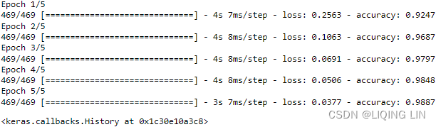
Two quantities are displayed during training:
- the loss of the network over the training data, and
- the accuracy of the network over the training data.
We quickly reach an accuracy of 0.989 (98.9%) on the training data. Now let’s check that the model performs well on the test set, too:
test_loss, test_acc = network.evaluate( test_images, test_labels )
print('test_loss:', test_loss)
print('test_acc:', test_acc)![]()
The test-set accuracy turns out to be 97.8%—that’s quite a bit lower than the training set accuracy. This gap between training accuracy and test accuracy is an example of overfitting: the fact that machine-learning models tend to perform worse on new data than on their training data. Overfitting is a central topic in chapter 3.
This concludes our first example—you just saw how you can build and train a neural network to classify handwritten digits in less than 20 lines of Python code. In the next chapter, I’ll go into detail about every moving piece we just previewed and clarify what’s going on behind the scenes. You’ll learn about tensors, the data-storing objects going into the network; tensor operations, which layers are made of; and gradient descent, which allows your network to learn from its training examples.
2.2 Data representations for neural networks
In the previous example, we started from data stored in multidimensional Numpy arrays, also called tensors. In general, all current machine-learning systems use tensors as their basic data structure. Tensors are fundamental to the field—so fundamental that Google’s TensorFlow was named after them. So what’s a tensor?
At its core, a tensor is a container for data—almost always numerical data. So, it’s a container for numbers. You may be already familiar with matrices, which are 2D tensors: tensors are a generalization of matrices to an arbitrary number of dimensions (note that in the context of tensors, a dimension is often called an axis).
2.2.1 Scalars (0D tensors)
x = np.array([12,3,6,14])
print(x)
print(x.ndim)
A tensor that contains only one number is called a scalar (or scalar tensor, or 0-dimensional tensor, or 0D tensor). In Numpy, a float32 or float64 number is a scalar tensor (or scalar array). You can display the number of axes of a Numpy tensor via the ndim attribute; a scalar tensor has 0 axes ( ndim == 0 ). The number of axes of a tensor is also called its rank. Here’s a Numpy scalar:
import numpy as np

x = np.array(12)

print(x)
print('x.dim:',x.ndim)![]()
2.2.2 Vectors (1D tensors)
An array of numbers is called a vector, or 1D tensor. A 1D tensor is said to have exactly one axis. Following is a Numpy vector:
x = np.array([12,3,6,14])
print(x)
print('x.dim:',x.ndim)![]()
This vector has five entries and so is called a 5-dimensional vector. Don’t confuse a 5D vector with a 5D tensor! A 5D vector has only 1 axis and has 5 dimensions along its axis, whereas a 5D tensor has 5 axes (and may have any number of dimensions along each axis).
Dimensionality can denote
- either the number of entries along a specific axis (as in the case of our 5D vector)
- or the number of axes in a tensor (such as a 5D tensor), which can be confusing at times.
In the latter case, it’s technically more correct to talk about a tensor of rank 5 (the rank of a tensor being the number of axes), but the ambiguous notation 5D tensor is common regardless.
2.2.3 Matrices (2D tensors)
An array of vectors is a matrix, or 2D tensor. A matrix has two axes (often referred to rows and columns). You can visually interpret a matrix as a rectangular grid of numbers. This is a Numpy matrix:
x = np.array([ [5, 78, 2, 34, 0],
               [6, 79, 3, 35, 1],
               [7, 80, 4, 36, 2]
             ])
print('x.ndim:', x.ndim)![]()
The entries from the first axis are called the rows, and the entries from the second axis are called the columns. In the previous example, [5, 78, 2, 34, 0] is the first row of x, and [5, 6, 7] is the first column
2.2.4 3D tensors and higher-dimensional tensors
If you pack such matrices in a new array, you obtain a 3D tensor, which you can visually interpret as a cube of numbers. Following is a Numpy 3D tensor:
import tensorflow as tf

x = np.array([ [5, 78, 2, 34, 0],
               [6, 79, 3, 35, 1],
               [7, 80, 4, 36, 2]
             ])# 2D

x_2D_tensor= tf.convert_to_tensor(x)
x_3D_tensor = tf.expand_dims(x_tensor, axis=0) # 3D # pack 2D
print(x_3D_tensor)
x_3D_tensor=tf.repeat( x_tensor,
                       repeats=[3], # The number of repetitions for each element.
                       axis=0,      # The axis along which to repeat values
                     )
print(x_3D_tensor)
print('ndim:',x_3D_tensor.ndim)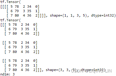
By packing 3D tensors in an array, you can create a 4D tensor, and so on. In deep learning, you’ll generally manipulate tensors that are 0D to 4D , although you may go up to 5D if you process video data.
2.2.5 Key attributes
A tensor is defined by three key attributes:
- Number of axes (rank)—For instance,
- a 3D tensor has three axes, and
- a matrix has two axes.
- This is also called the tensor’s ndim in Python libraries such as Numpy.
- Shape—This is a tuple of integers that describes how many dimensions the tensor has along each axis. For instance,
- the previous matrix example has shape (3, 5) ,
- and the 3D tensor example has shape (3, 3, 5) .
- A vector has a shape with a single element, such as (5,) , whereas
- a scalar has an empty shape, () .
- Data type (usually called dtype in Python libraries)—This is the type of the data contained in the tensor;
x_3D_tensor.dtype
- for instance, a tensor’s type could be float32 , uint8 , float64 , and so on. On rare occasions, you may see a char tensor. Note that string tensors don’t exist in Numpy (or in most other libraries), because tensors live in pre-allocated, contiguous memory segments: and strings, being variable length, would preclude the use of this implementation.
Let’s display the fourth digit in the 3D tensor, using the library Matplotlib (part of the standard scientific Python suite); see figure 2.2.
(train_images, train_labels), (test_images, test_labels) = mnist.load_data()
#Listing 2.6 Displaying the fourth digit
digit = train_images[4]
import matplotlib.pyplot as plt
plt.imshow( digit, cmap=plt.cm.binary )
plt.show()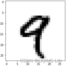 Figure 2.2 The fourth sample in our dataset
2.2.8 Real-world examples of data tensors
Let’s make data tensors more concrete with a few examples similar to what you’ll encounter later. The data you’ll manipulate will almost always fall into one of the following categories:
- Vector data— 2D tensors of shape (samples, features)
This is the most common case. In such a dataset, each single data point can be encoded as a vector, and thus a batch of data will be encoded as a 2D tensor (that is, an array of vectors), where the first axis is the samples axis and the second axis is the features axis.
Let’s take a look at two examples:- An actuarial/ˌæktʃuˈeəriəl/保险精算的 dataset of people, where we consider each person’s age, ZIP code, and income. Each person can be characterized as a vector of 3 values, and thus an entire dataset of 100,000 people can be stored in a 2D tensor of shape (100000, 3)
- A dataset of text documents, where we represent each document by the counts of how many times each word appears in it (out of a dictionary of 20,000 common words). Each document can be encoded as a vector of 20,000 values (one count per word in the dictionary), and thus an entire dataset of 500 documents can be stored in a tensor of shape (500, 20000)
- Timeseries data or sequence data— 3D tensors of shape (samples, timesteps, features)
Whenever time matters in your data (or the notion of sequence order), it makes sense to store it in a 3D tensor with an explicit time axis. Each sample can be encoded as a sequence of vectors (a 2D tensor), and thus a batch of data will be encoded as a 3D tensor (see figure 2.3).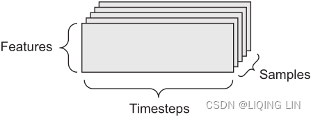 Figure 2.3 A 3D timeseries data tensor
The time axis is always the second axis (axis of index 1), by convention. Let’s look at a
few examples:- A dataset of stock prices. Every minute, we store the current price of the stock, the highest price in the past minute, and the lowest price in the past minute. Thus every minute is encoded as a 3D vector, an entire day of trading is encoded as a 2D tensor of shape (390, 3) (there are 390 minutes in a trading day), and 250 days’ worth of data can be stored in a 3D tensor of shape (250, 390, 3) . Here, each sample would be one day’s worth of data.
- A dataset of tweets, where we encode each tweet as a sequence of 280 characters out of an alphabet of 128 unique characters. In this setting, each character can be encoded as a binary vector of size 128 (an all-zeros vector except for a 1 entry at the index corresponding to the character). Then each tweet can be encoded as a 2D tensor of shape (280, 128) , and a dataset of 1 million tweets can be stored in a tensor of shape (1000000, 280, 128)
- Images— 4D tensors of shape (samples, height, width, channels) or (samples, channels, height, width)
Images typically have three dimensions: height, width, and color depth. Although grayscale images (like our MNIST digits) have only a single color channel and could thus be stored in 2D tensors, by convention image tensors are always 3D , with a one-dimensional color channel for grayscale images. A batch of 128 grayscale images of size 256 × 256 could thus be stored in a tensor of shape (128, 256, 256, 1) , and a batch of 128 color images could be stored in a tensor of shape (128, 256, 256, 3) (see figure 2.4).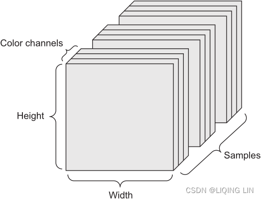 Figure 2.4 A 4D image data tensor (channels-first convention)
There are two conventions for shapes of images tensors: the channels-last convention (used by TensorFlow) and the channels-first convention (used by Theano). The Tensor-Flow machine-learning framework, from Google, places the color-depth axis at the end: (samples, height, width, color_depth) . Meanwhile, Theano places the color depth axis right after the batch axis: (samples, color_depth, height, width) . With the Theano convention, the previous examples would become (128, 1, 256, 256) and (128, 3, 256, 256) . The Keras framework provides support for both formats. - Video— 5D tensors of shape (samples, frames, height, width, channels) or (samples, frames, channels, height, width)
Video data is one of the few types of real-world data for which you’ll need 5D tensors. A video can be understood as a sequence of frames, each frame being a color image. Because each frame can be stored in a 3D tensor (height, width, color_depth) , a sequence of frames can be stored in a 4D tensor (frames, height, width, color_depth) , and thus a batch of different videos can be stored in a 5D tensor of shape (samples, frames, height, width, color_depth).
For instance, a 60-second, 144 × 256 YouTube video clip sampled at 4 frames per second would have 240 frames. A batch of four such video clips would be stored in a tensor of shape (4, 240, 144, 256, 3) . That’s a total of 106,168,320 values! If the dtype of the tensor was float32 , then each value would be stored in 32 bits, so the tensor would represent 405 MB. Heavy! Videos you encounter in real life are much lighter, because they aren’t stored in float32 , and they’re typically compressed by a large factor (such as in the MPEG format).
2.3 tensor operations
Much as any computer program can be ultimately reduced to a small set of binary operations on binary inputs ( AND , OR , NOR , and so on), all transformations learned by deep neural networks can be reduced to a handful of tensor operations applied to tensors of numeric data. For instance, it’s possible to add tensors, multiply tensors, and so on.
2.3.2 Broadcasting
Our earlier naive implementation of naive_add only supports the addition of 2D tensors with identical shapes. But in the Dense layer introduced earlier, we added a 2D tensor with a vector. What happens with addition when the shapes of the two tensors being added differ?
When possible, and if there’s no ambiguity, the smaller tensor will be broadcasted to match the shape of the larger tensor. Broadcasting consists of two steps:
- 1 Axes (called broadcast axes) are added to the smaller tensor to match the ndim of the larger tensor.
- 2 The smaller tensor is repeated alongside these new axes to match the full shape of the larger tensor.
Let’s look at a concrete example. Consider X with shape (32, 10) and y with shape (10,) .
- First, we add an empty first axis to y , whose shape becomes (1, 10) .
- Then, we repeat y 32 times alongside this new axis, so that we end up with a tensor Y with shape (32, 10) , where Y[i, :] == y for i in range(0, 32) . At this point, we can proceed to add X and Y , because they have the same shape.
In terms of implementation, no new 2D tensor is created, because that would be terribly inefficient. The repetition operation is entirely virtual: it happens at the algorithmic level rather than at the memory level. But thinking of the vector being repeated 10 times alongside a new axis is a helpful mental model. Here’s what a naive implementation would look like:
With broadcasting, you can generally apply two-tensor element-wise operations if one tensor has shape (a, b, … n, n + 1, … m) and the other has shape (n, n + 1, … m) . The broadcasting will then automatically happen for axes a through n - 1.
The following example applies the element-wise maximum operation to two tensors of different shapes via broadcasting: 
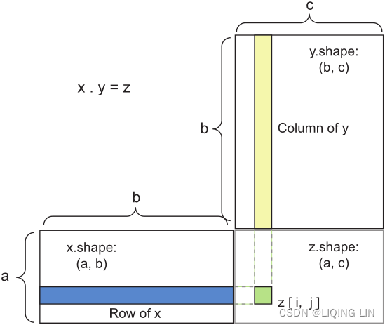 Figure 2.5 Matrix dot-product box diagram


 2396
2396


 被折叠的 条评论
为什么被折叠?
被折叠的 条评论
为什么被折叠?
 到【灌水乐园】发言


