


Graphs can be used to represent a wide range of phenomena. This is particularly true for online social networks, and the Internet of Things (IoT). Graph mining is big business, with websites such as Facebook running on data analysis experiments performed on graphs.
Social media websites are built upon engagement[ɪnˈɡeɪdʒmənt]参与度 . Users without active news feeds, or interesting friends to follow, do not engage with sites. In contrast, users with more interesting friends and followees关注者 engage more, see more ads. This leads to larger revenue streams for the website.
In this chapter, we look at how to define similarity on graphs, and how to use them within a data mining context. Again, this is based on a model of the phenomena. We look at some basic graph concepts, like sub-graphs and connected components. This leads to an investigation of cluster analysis, which we delve more deeply into in Chapter 10"," Clustering News Articles.
The topics covered in this chapter include:
- Clustering data to find patterns
- Loading datasets from previous experiments
- Getting follower information from Twitter
- Creating graphs and networks
- Finding subgraphs for cluster analysis
Loading the dataset
In this chapter, our task is to recommend users on online social networks based on shared connections. Our logic is that if two users have the same friends, they are highly similar and worth recommending to each other. We want our recommendations to be of high value. We can only recommend so many people before it becomes tedious, therefore we need to find recommendations that engage users.
To do this, we use the previous chapter's disambiguation model to find only users talking about Python as a programming language. In this chapter, we use the results from one data mining experiment as input into another data mining experiment. Once we have our Python programmers selected, we then use their friendships to find clusters of users that are highly similar to each other. The similarity between two users will be defined by how many friends they have in common. Our intuition will be that the more friends two people have in common, the more likely two people are to be friends (and therefore should be on our social media platform).
We are going to create a small social graph from Twitter using the API we introduced in the previous chapter. The data we are looking for is a subset of users interested in a similar topic (again, the Python programming language) and a list of all of their friends (people they follow关注的人). With this data, we will check how similar two users are, based on how many friends they have in common.
There are many other online social networks apart from Twitter. The reason we have chosen Twitter for this experiment is that their API makes it quite easy to get this sort of information. The information is available from other sites, such as Facebook, LinkedIn, and Instagram, as well. However, getting this information is more difficult.
To start collecting data, set up a new Jupyter Notebook and an instance of the twitter connection, as we did in the previous chapter. You can reuse the app information from the previous chapter or create a new one:
import twitter

# API Key and Secret
consumer_key = 'HW5MoQ6BfFVZhhV5IahfhNQXV'
consumer_secret = 'ouzrDgvdZOpa7AFdcrYrRKezNWaTN5p08JeU9UdnOnnyNsl0KI'
# Access Token and Secret
access_token = '1441908129701138436-trVsSMGs518y9hvRS8dmMBrCXlzPsE'
access_token_secret = 'QasEX8VSD1oN1FwRQgNIIBcrh3alC8sVKiG3ofgOUD9JI'

authorization = twitter.OAuth( access_token, access_token_secret,
                               consumer_key, consumer_secret
                             )
Also, set up the filenames. You will want to use a different folder for this experiment from the one you used in m06_Social Media twitter Using Naive Bayes_PermissionError [Errno 13]_NLP_bag词袋_Ngram_spaCy_pipeline_Linli522362242的专栏-CSDN博客, ensuring you do not override your previous dataset!
import os

# PermissionError: [Errno 13] Permission denied: 'dataset/twitter/python_tweets.json'
#                  path = os.path.join( '/'.join(["dataset","twitter", "python_tweets.json"]) )
#                  since python_tweets.json is a folder after os.makedir(path) instead of a json file
# solution:
path = os.path.join( '/'.join(["dataset","twitter", "m07"]) )
if not os.path.exists( path ):
    os.mkdir(path)
output_filename = path + "/python_tweets.json"
output_filename![]()

Next, we will need a list of users. We will do a search for tweets, as we did in the previous chapter, and look for those mentioning the word python. First, create 2 lists for storing the tweet's text and the corresponding users. We will need the user IDs later, so we create a dictionary mapping that now. The code is as follows:
original_users = [] # user's screen_name
tweets = []
user_ids = {} # user's screen_name : user's id
We will now perform a search for the word python, as we did in the m06_Social Media twitter Using Naive Bayes_PermissionError [Errno 13]_NLP_bag词袋_Ngram_spaCy_pipeline_Linli522362242的专栏-CSDN博客, and iterate over the search results and only saving Tweets with text (as per the last chapter's requirements):
t = twitter.Twitter( auth=authorization, retry=True )
search_results = t.search.tweets( q='python', count=100 )['statuses']

search_results[0]
# run this to get more tweets # step1

# run this to get more tweets # step2
for tweet in search_results:
    if 'text' in tweet:
        original_users.append( tweet['user']['screen_name'] )
        user_ids[ tweet['user']['screen_name'] ] = tweet['user']['id']
        tweets.append( tweet['text'] )
user_ids
len(tweets) ![]() Running this code will get about 100 tweets, maybe a little fewer in some cases. Not all of them will be related to the programming language, though. We will address that by using the model we trained in the m06_Social Media twitter Using Naive Bayes_PermissionError [Errno 13]_NLP_bag词袋_Ngram_spaCy_pipeline_Linli522362242的专栏-CSDN博客
Running this code will get about 100 tweets, maybe a little fewer in some cases. Not all of them will be related to the programming language, though. We will address that by using the model we trained in the m06_Social Media twitter Using Naive Bayes_PermissionError [Errno 13]_NLP_bag词袋_Ngram_spaCy_pipeline_Linli522362242的专栏-CSDN博客
tweet_filename = os.path.join('dataset/twitter/recreate/test_tweets.json')
with open(tweet_filename, 'a') as output_file:
    for tweet in tweets:
        output_file.write( json.dumps(tweet) )
        output_file.write("\n\n")
tweet_filename = os.path.join('dataset/twitter/recreate/test_tweets.json')
tweet_test = []
with open( tweet_filename ) as inputFile:
for line in inputFile:
if len( line.strip() ) == 0:
continue
tweet_test.append( json.loads(line) )
len(tweet_test)![]()
users_filename = os.path.join('dataset/twitter/recreate/test_users_tweets.json')
with open(users_filename, 'a') as output_file:
for user in original_users:
output_file.write( json.dumps(user) )
output_file.write("\n\n")
users_filename = os.path.join('dataset/twitter/recreate/test_users_tweets.json')
users = []
with open( users_filename ) as inputFile:
for line in inputFile:
if len( line.strip() ) == 0:
continue
users.append( json.loads(line) )
len(users) ![]()
user_id_filename = os.path.join('dataset/twitter/recreate/test_user_id_tweets.json')
with open(user_id_filename, 'a') as output_file:
output_file.write( json.dumps(user_ids) )
user_id_filename = os.path.join('dataset/twitter/recreate/test_user_id_tweets.json')
user_id_dict = None
with open(user_id_filename) as inputFile:
user_id_dict = json.load( inputFile )
user_id_dict 
len( user_id_dict.keys() ), len( user_id_dict.values() ), len( set(users) ), len(users) ![]() A user may post multiple tweets
A user may post multiple tweets
len( user_ids.keys() ), len( user_ids.values() ), len( set(original_users) ), len(original_users) ![]() A user may post multiple tweets
A user may post multiple tweets
len( set(tweet_test) ), len( tweet_test ) ![]()
and a user’s tweet may be copied and pasted directly by other users.
Classifying with an existing model
In this case, we are only interested in users who are tweeting about Python, the programming language. We will use our classifier from the last chapter to determine which tweets are related to the programming language. From there, we will select only those users who were tweeting about the programming language.
To do this part of our broader experiment, we first need to save the model from the previous chapter. Open the Jupyter Notebook we made in the last chapter, the one in which we built and trained the classifier.
If you have closed it, then the Jupyter Notebook won't remember what you did, and you will need to run the cells again. To do this, click on the Cell menu on the Notebook and choose Run All.
import spacy
from sklearn.base import TransformerMixin
import string
import nltk
# Create a spaCy parser
nlp = spacy.load('en_core_web_sm')
class BagOfWords( TransformerMixin ):
def fit( self, X, y=None ):
return self
def transform( self, X ):
results = [] # a list of dictionaries
for document in X:
row = {}
texts = " ".join( "".join( [" " if ch in string.punctuation else ch
for ch in document
]# Removal of punctuations or replace all punctuations with blank
).split() # return a word_array or remove "\n"
) # outer join for recreating an new paragraph excluding "\n"
# step2 # Return a sentence-tokenized copy of text # In fact, it’s not needed here, just to show
tokens = [ word for sent in nltk.sent_tokenize( texts )
for word in nltk.word_tokenize(sent)
] # Return a tokenized copy of text
# stopwds = stopwords.words('english')
# tokens = [token for token in tokens
# if token not in stopwds
# ]# step4 Stop word removal
# #stemmer = PorterStemmer()
# tokens = [ stemmer.stem(word) for word in tokens ] # step 6 Stemming of words
for word in tokens:
row[word] = True
results.append( row )
return resultsfrom sklearn.feature_extraction import DictVectorizer
from sklearn.naive_bayes import BernoulliNB
import os
# PermissionError: [Errno 13] Permission denied: 'dataset/twitter/python_tweets.json'
# path = os.path.join( '/'.join(["dataset","twitter", "python_tweets.json"]) )
# since python_tweets.json is a folder after os.makedir(path) instead of a json file
# solution:
path = os.path.join( '/'.join(["dataset","twitter", "recreate"]) )
if not os.path.exists( path ):
os.mkdir(path)
tweet_filename = path + "/python_tweets.json"
labels_filename = path + '/replicable_python_classes.json'
import json
tweets = []
with open( tweet_filename ) as inputFile:
for line in inputFile:
if len( line.strip() ) == 0:
continue
tweets.append( json.loads(line)['text'] )
with open( labels_filename ) as inputFile:
labels = json.load( inputFile )
# Ensure only classified tweets are loaded
tweets = tweets[:len(labels)]
assert len(tweets) == len(labels)
len(tweets), len(labels) ![]()
from sklearn.pipeline import Pipeline
pipeline = Pipeline( [( 'bag-of-words', BagOfWords() ),
( 'vectorizer', DictVectorizer() ),
( 'naive-bayes', BernoulliNB() )
] )
from sklearn.model_selection import cross_val_score
scores = cross_val_score( pipeline, tweets, labels, scoring='f1' )# cv=5 : default 5-fold
import numpy as np
print( 'Score: {:.3f}'.format( np.mean(scores) ) ) ![]()
model = pipeline.fit( tweets, labels )
# pipeline gives you access to the individual steps through the named_steps attribute
# and the name of the step
nb = model.named_steps['naive-bayes']
# extract the probabilities for each word. These are stored as log probabilities,
# which is simply log(P(A|f)), where f is a given feature
feature_probabilities = nb.feature_log_prob_
top_features = np.argsort( -nb.feature_log_prob_[1])[:50]
# dv: DictVectorizer
dv = model.named_steps['vectorizer']
for i, feature_index in enumerate(top_features):
print(i, dv.feature_names_[feature_index], #########
np.exp( feature_probabilities[1][feature_index] )
)
feature_probabilities.shape![]()
We are going to use the joblib library to save our model and load it.
joblib is included with the scikit-learn package as a built-in external package. No extra installation step needed! This library has tools for saving and loading models, and also for simple parallel processing - which is used in scikit-learn quite a lot.
os.getcwd() ![]()
import joblib
path = os.path.join( '/'.join(["models","twitter"]) )
if not os.path.exists( path ):
for p in path.split('/'):
deeper_path = os.path.join( os.getcwd(), p )
print(deeper_path)
if not os.path.exists(deeper_path):
os.mkdir(deeper_path)
os.chdir(deeper_path)
else:
os.chdir(deeper_path)
continue
else:
os.chdir(path)
# tweet_filename = path + "/python_tweets.json"
# labels_filename = path + '/replicable_python_classes.json'
os.getcwd()
output_model_filename = "python_context.pkl"
output_model_filename ![]()
Next, we use the dump function in joblib, which works much like the similarly named version in the json library. We pass the model itself and the output filename:
joblib.dump( model, output_model_filename )![]()

#################################### Return to the upper level directory
os.getcwd()![]()
os.path.abspath( os.path.join( os.path.dirname("__file__"),os.path.pardir) ) ![]()
os.chdir(
os.path.abspath( os.path.join( os.path.dirname("__file__"),os.path.pardir) )
)
os.chdir(
os.path.abspath( os.path.join( os.path.dirname("__file__"),os.path.pardir) )
)
os.getcwd() ![]()
####################################
load this model
import joblib
path = os.path.join( '/'.join(["models","twitter"]) )
output_model_filename = path+"/python_context.pkl"
context_classifier_forTweet = joblib.load(output_model_filename)
![]()
![]()
AttributeError: module '__main__' has no attribute 'BagOfWords'
we need to recreate our BagOfWords class, as it was a custom-built class and can't be loaded directly by joblib. Simply copy the entire BagOfWords class from the previous chapter's code, including its dependencies:
import spacy
from sklearn.base import TransformerMixin
import string
import nltk
# Create a spaCy parser
nlp = spacy.load('en_core_web_sm')
class BagOfWords( TransformerMixin ):
def fit( self, X, y=None ):
return self
def transform( self, X ):
results = [] # a list of dictionaries
for document in X:
row = {}
texts = " ".join( "".join( [" " if ch in string.punctuation else ch
for ch in document
]# Removal of punctuations or replace all punctuations with blank
).split() # return a word_array or remove "\n"
) # outer join for recreating an new paragraph excluding "\n"
# step2 # Return a sentence-tokenized copy of text # In fact, it’s not needed here, just to show
tokens = [ word for sent in nltk.sent_tokenize( texts )
for word in nltk.word_tokenize(sent)
] # Return a tokenized copy of text
# stopwds = stopwords.words('english')
# tokens = [token for token in tokens
# if token not in stopwds
# ]# step4 Stop word removal
# #stemmer = PorterStemmer()
# tokens = [ stemmer.stem(word) for word in tokens ] # step 6 Stemming of words
for word in tokens:
row[word] = True
results.append( row )
return resultsIn production, you would need to develop your custom transformers in separate, centralized files, and import them into the Notebook instead. This little hack simplifies the workflow, but feel free to experiment with centralizing important code by creating a library of common functionality.
Loading the model now just requires a call to the load function of joblib:
load this model again
import joblib
path = os.path.join( '/'.join(["models","twitter"]) )
output_model_filename = path+"/python_context.pkl"
context_classifier_forTweet = joblib.load(output_model_filename) ![]()
![]()
Our context_classifier is an instance of a Pipeline, with the same three steps as before (BagOfWords, DictVectorizer, and a BernoulliNB classifier). Calling the predict function on this model gives us a prediction as to whether our tweets are relevant to the programming language. The code is as follows:
y_pred = context_classifier_forTweet.predict( tweets )
y_pred If the results you get are all 0, you may need to use Twitter api multiple times to get data in this case
len(tweets)![]()
###################################
# if you have the tweet_tests.json file
tweet_filename = os.path.join('dataset/twitter/recreate/test_tweets.json')
tweet_test = []

with open( tweet_filename ) as inputFile:
    for line in inputFile:
        if len( line.strip() ) == 0:
            continue
        tweet_test.append( json.loads(line) )
len(tweet_test)![]()
###################################
Save to local drive( # run this to get more tweets # step3)
tweet_filename = os.path.join('dataset/twitter/recreate/test_tweets.json')
with open(tweet_filename, 'a') as output_file:
    for tweet in tweets:
        output_file.write( json.dumps(tweet) )
        output_file.write("\n\n")
read tweet from local drive
tweet_filename = os.path.join('dataset/twitter/recreate/test_tweets.json')
tweet_test = []

with open( tweet_filename ) as inputFile:
    for line in inputFile:
        if len( line.strip() ) == 0:
            continue
        tweet_test.append( json.loads(line) )
len(tweet_test) ![]()
The ith item in y_pred will be 1 if the ith tweet is (predicted to be) related to the programming language, or else it will be 0. From here, we can get just the tweets that are relevant and their relevant users:
relevant_tweets = [ tweets[i]
                    for i in range( len(tweets) )
                       if y_pred[i] == 1
                  ]
relevant_user = [ original_users[i]# tweet['user']['screen_name']
                     for i in range( len(tweets) )
                        if y_pred[i]== 1
                ]# original_users ~ user_ids ~ tweet['text']
len(relevant_tweets), len(relevant_user)![]()
Using my data, this comes up to 48 relevant users. now we have a basis for building our social network. We can always add more data to get more users, but 48 users will be sufficient to go through this chapter as a first pass. I recommend coming back, adding more data, and running the code again, to see what results you obtain.
Getting follower information from Twitter
With our initial set of users, we now need to get the friends of each of these users. A friend is a person whom the user is following. The API for this is called friends/ids, and it has both good and bad points. The good news is that it returns up to 5,000 friend IDs in a single API call. The bad news is that you can only make 15 calls every 15 minutes, which means it will take you at least 1 minute per user to get all followers—more if they have more than 5,000 friends (which happens more often than you may think).
The code is similar to the code from our previous API usage (obtaining tweets). We will package it as a function, as we will use this code in the next two sections. Our function takes a twitter user's ID value, and returns their friends. While it may be surprising to some, many Twitter users have more than 5,000 friends. Due to this we will need to use Twitter's pagination function, which lets Twitter return multiple pages of data through separate API calls. When you ask Twitter for information, it gives you your information along with a cursor, which is an integer that Twitter uses to track your request. If there is no more information, this cursor is 0; otherwise, you can use the supplied cursor to get the next page of results. Passing this cursor lets twitter continue your query, returning the next set of data to you.
In the function, we keep looping while this cursor is not equal to 0 (as, when it is, there is no more data to collect). We then perform a request for the user's followers and add them to our list. We do this in a try block, as there are possible errors that can happen that we can handle. The follower's IDs are stored in the ids key of the results dictionary. After obtaining that information, we update the cursor. It will be used in the next iteration of the loop. Finally, we check if we have more than 10,000 friends. If so, we break out of the loop. The code is as follows:
https://developer.twitter.com/en/docs/twitter-api/v1/accounts-and-users/follow-search-get-users/api-reference/get-friends-ids
import time

def get_friends( t, user_id ):
    friends = []
    cursor = -1
    while cursor != 0:
        try:
            results = t.friends.ids( user_id = user_id, cursor= cursor, count=5000 )
            friends.extend([ friend for friend in results['ids'] ])
            cursor = results['next_cursor']
            if True or len(friends)>=10000:
                break
        except TypeError as e:
            if results is None:
                print("You probably reached your API limit, waiting for 5 minutes")
                sys.stdout.flush()
                time.sleep( 5*60 ) # 5 minute wait
            else:
                # Some other error happened, so raise the error as normal
                raise e
        except twitter.TwitterHTTPError as e:
            print(e)
            break
        finally:
            # Break regardless -- this stops us going over our API limit
            time.sleep(60)
    return friends
It is worth inserting a warning here. We are dealing with data from the Internet, which means weird things can and do happen regularly. A problem I ran into when developing this code was that some users have many, many, many thousands of friends. As a fix for this issue, we will put a failsafe here, exiting the function if we reach more than 10,000 users. If you want to collect the full dataset, you can remove these lines, but beware that it may get stuck on a particular user for a very long time.
Much of the above function is error handling, as quite a lot can go wrong when dealing with external APIs!
The most likely error that can happen is if we accidentally reach our API limit (while we have a sleep to stop that, it can occur if you stop and run your code before this sleep finishes). In this case, results is None and our code will fail with a TypeError. In this case, we wait for 5 minutes and try again, hoping that we have reached our next 15-minute window. There may be another TypeError that occurs at this time. If one of them does, we raise it and will need to handle it separately.
The second error that can happen occurs at Twitter's end, such as asking for a user that doesn't exist or some other data-based error, resulting in a TwitterHTTPError (which is a similar concept to a HTTP 404 error). In this case, don't try this user anymore, and just return any followers we did get (which, in this case, is likely to be 0).
Finally, Twitter only lets us ask for follower information 15 times every 15 minutes, so we will wait for 1 minute before continuing. We do this in a finally block so that it happens even if an error occurs.
Building the network
Now we are going to build our network of users, where users are linked if the two users follow each other. The aim of building this network is to give us a data structure we can use to segment our list of users into groups. From these groups, we can then recommend people in the same group to each other. Starting with our original users, we will get the friends for each of them and store them in a dictionary. Using this concept we can grow the graph outwards from an initial set of users.
Starting with our original users, we will get the friends for each of them and store them in a dictionary (after obtaining the user's ID from our user_id dictionary):
friends = {}
for screen_name in relevant_user:#[:50]:
    user_id = user_ids[screen_name]
    friends[user_id] = get_friends(t, user_id)

friends
len(friends), len(friends.keys())![]()
id_friendsID_filename = os.path.join('dataset/twitter/recreate/id_friendsID_tweets.json')
with open(id_friendsID_filename, 'a') as output_file:
output_file.write( json.dumps(friends) )![]()
id_friendsID_filename = os.path.join('dataset/twitter/recreate/id_friendsID_tweets.json')
id_friendsID_dict = None
with open(id_friendsID_filename) as inputFile:
    id_friendsID_dict = json.load( inputFile )

id_friendsID_dict
Next, we are going to remove any user who doesn't have any friends. For these users, we can't really make a recommendation in this way. Instead, we might have to look at their content or people who follow them. We will leave that out of the scope of this chapter, though, so let's just remove these users. The code is as follows:
friends = id_friendsID_dict
friends = { user_id:friends[user_id]
            for user_id in friends
              if len(friends[user_id])>0
          }
len(friends)![]()
We now have between 30 and 50 users, depending on your initial search results. We are now going to increase that amount to 150. The following code will take quite a long time to run—given the limits on the API, we can only get the friends for a user once every minute. Simple math will tell us that 150 users will take 150 minutes, which is at least 2 hours and 30 minutes. Given the time we are going to be spending on getting this data, it pays to ensure we get only good users.
To do this, we simply iterate over all the friend lists we have and then count each time a friend occurs.
from collections import defaultdict

def count_friends( friends ):
    friend_count = defaultdict(int)

    for friend_list in friends.values():
        for friend in friend_list:
            friend_count[friend] += 1
    return friend_count
Computing our current friend count, we can then get the most connected (that is, most friends from our existing list) person from our sample. The code is as follows:
friend_count = count_friends(friends)
friend_count 
sort dict by value
from operator import itemgetter

sorted( friend_count.items(), key=lambda friend_count:friend_count[1], reverse=True ) 
sort dict by value and return a reversed key list
from operator import itemgetter

best_friends = sorted( friend_count, key=friend_count.get, reverse=True )
best_friends 
From here, we set up a loop that continues until we have the friends of 150 users. We then iterate over all of our best friends (which happens in order of the number of people who have them as friends) until we find a user we have not yet checked. We then get the friends of that user and update the friends counts. Finally, we work out who is the most connected user who we haven't already got in our list:
import sys
# t = twitter.Twitter( auth=authorization, retry=True )
while len(friends) < 150:
    for friend_user_id in best_friends:
        if friend_user_id in friends:# key is current user id
            continue
        #else:
        print( friend_user_id )
        sys.stdout.flush()
        friends[friend_user_id] = get_friends( t, friend_user_id ) # append to friends

        for friend in friends[friend_user_id]: #
            friend_count[friend] +=1
        best_friends = sorted(friend_count, key=friend_count.get, reverse=True)
        break
The codes will then loop and continue until we reach 150 users.
You may want to set these value lower, such as 40 or 50 users (or even just skip this bit of code temporarily). Then, complete the chapter's code and get a feel for how the results work. After that, reset the number of users in this loop to 150, leave the code to run for a few hours, and then come back and rerun the later code.
Given that collecting that data probably took over 2 hours, it would be a good idea to save it in case we have to turn our computer off. Using the json library, we can easily save our friends dictionary to a file:
id_friendsID_150 = os.path.join('dataset/twitter/recreate/id_friendsID_150.json')
with open(id_friendsID_150, 'a') as output_file:
     output_file.write( json.dumps(friends) )
If you need to load the file, use the json.load function:
id_friendsID_150 = os.path.join('dataset/twitter/recreate/id_friendsID_150.json')
id_friendsID_150dict = None
with open(id_friendsID_150) as inputFile:
    id_friendsID_150dict = json.load( inputFile )

id_friendsID_150dict
len(friends), len(id_friendsID_150dict), \
len(friends.keys()), len(id_friendsID_150dict.keys()), \
len(friends.values()), len(id_friendsID_150dict.values()), ![]()
friend_count_150 = os.path.join('dataset/twitter/recreate/friend_count_150.json')
with open(friend_count_150, 'a') as output_file:
     output_file.write( json.dumps(friend_count) )
friend_count_150 = os.path.join('dataset/twitter/recreate/friend_count_150.json')
friend_count_150_dict = None
with open(friend_count_150) as inputFile:
friend_count_150_dict = json.load( inputFile )
friend_count_150_dict
best_friends = sorted(friend_count_150_dict, key=friend_count_150_dict.get, reverse=True)
len( best_friends ), best_friends[:5] 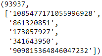
sorted(friend_count_150_dict.items(), key=itemgetter(1), reverse=True)
Creating a graph
Now, we have a list of users and their friends and many of these users are taken from friends of other users. This gives us a graph where some users are friends of other users (although not necessarily the other way around).
A graph is a set of nodes and edges. Nodes are usually objects—in this case, they are our users. The edges in this initial graph indicate that user A is a friend of user B. We call this a directed graph, as the order of the nodes matters. Just because user A is a friend of user B, that doesn't imply that user B is a friend of user A. The example network below shows this, along with a user C who is friends of user B, and is friended in turn by user B as well. We can visualize this graph using the NetworkX package.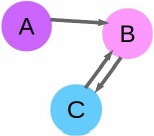
Once again, you can use Anaconda to install NetworkX:https://blog.csdn.net/Linli522362242/article/details/108037567
conda install networkx 
First, we create a directed graph using NetworkX. By convention, when importing NetworkX, we use the abbreviation nx (although this isn't necessary). The code is as follows:
import networkx as nx

G = nx.DiGraph()
We will only visualize our key users, not all of the friends (as there are many thousands of these and it is hard to visualize). We get our main users and then add them to our graph as nodes:
main_users = id_friendsID_150dict.keys()
G.add_nodes_from( main_users )
Next we set up the edges. We create an edge from a user to another user if the second user is a friend of the first user. To do this, we iterate through all of the friends of a given user. We ensure that the friend is one of our main users (as we currently aren't interested in visualizing the other users), and add the edge if they are.
for main_user_id in id_friendsID_150dict:
    for friend in id_friendsID_150dict[main_user_id]:
        if str( friend ) in main_users:
            G.add_edge( main_user_id, friend )
We can now visualize the network using NetworkX's draw function, which uses matplotlib. To get the image in our notebook, we use the inline function on matplotlib and then call the draw function. The code is as follows:
%matplotlib inline

nx.draw(G)
The results are a bit hard to make sense of; they show that there are some nodes with few connections but many nodes with many connections: 
We can make the graph a bit bigger by using pyplot to handle the creation of the figure. To do that, we import pyplot, create a large figure, and then call NetworkX's draw function (NetworkX uses pyplot to draw its figures):
from matplotlib import pyplot as plt

plt.figure( 3, figsize=(20,20) )
nx.draw(G, alpha=0.1, edge_color='b')
As you can see, it is very well connected in the center!
The results are too big for a page here, but by making the graph bigger, an outline of how the graph appears can now be seen. In my graph, there was a group users all highly connected to each other, and most other users didn't have many connections at all. I have zoomed in on just the center of the network here and set the edge color to blue with a low alpha(alpha=0.1) in the preceding code.
This is actually a property of our method of choosing new users—we choose those who are already well linked in our graph, so it is likely they will just make this group larger. For social networks, generally the number of connections a user has follows a power law. A small percentage of users have many connections, and others have only a few. The shape of the graph is often described as having a long tail. Our dataset doesn't follow this pattern, as we collected our data by getting friends of users we already had.
Creating a similarity graph
Our task in this chapter is recommendation through shared friends. As mentioned previously, our logic is that, if two users have the same friends, they are highly similar. We could recommend one user to the other on this basis.
We are therefore going to take our existing graph (which has edges relating to friendship) and create a new graph. The nodes are still users, but the edges are going to be weighted edges. A weighted edge is simply an edge with a weight property. The logic is that a higher weight indicates more similarity between the two nodes than a lower weight. This is context-dependent. If the weights represent distance, then the lower weights indicate more similarity.
For our application, the weight will be the similarity of the two users connected by that edge (based on the number of friends they share). This graph also has the property that it is not directed. This is due to our similarity computation, where the similarity of user A to user B is the same as the similarity of user B to user A.
There are many ways to compute the similarity between two lists like this. For example, we could compute the number of friends the two have in common. However, this measure is always going to be higher for people with more friends Instead, we can normalize it by dividing by the total number of distinct friends the two have. This is called the Jaccard Similarity.
Other similarity measurements are directed. An example is ratio of similar users, which is the number of friends in common divided by the user's total number of friends. In this case, you would need a directed graph.
The Jaccard Similarity, always between 0 and 1, represents the percentage overlap of the two两者. As we saw in Chapter 2, Classifying with scikit-learn Estimators, normalization is an important part of data mining exercises and generally a good thing to do (unless you have a specific reason not to).
To compute the Jaccard similarity, we divide the intersection of the two sets of followers by the union of the two. These are set operations and we have lists, so we will need to convert the friends lists to sets first. The code is as follows:
friends = { main_user_id: set( id_friendsID_150dict[main_user_id] )
               for main_user_id in id_friendsID_150dict
          }
We then create a function that computes the similarity of two sets of friends lists. The code is as follows:
def compute_similarity( friends1, friends2 ):
    return len( friends1 & friends2) / ( len( friends1 | friends2) + 1e-6 )
OR
def compute_similarity( friends1, friends2 ):
    return len( friends1.intersection(friends2) ) / ( len( friends1.union(friends2) ) + 1e-6 )
We add 1e-6 (or 0.000001) to the similarity above to ensure we never get a division by zero error, in cases where neither user has any friends. It is small enough to not really affect our results, but big enough to be more than zero.
From here, we can create our weighted graph of the similarity between users. We will use this quite a lot in the rest of the chapter, so we will create a function to perform this action. Let's take a look at the threshold parameter (directly dictates how many connected components we discover and how big they are):
def create_graph( followers, threshold=0 ):
    # https://networkx.org/documentation/stable/tutorial.html
    G = nx.Graph()
    for user1 in friends.keys():
        for user2 in friends.keys():
            if user1 == user2:
                continue
            # else:
            weight = compute_similarity( friends[user1],
                                         friends[user2] )
            if weight >= threshold:
                G.add_node( user1 )
                G.add_node( user2 )
                G.add_edge( user1, user2, weight=weight )###########
    return G
We can now create a graph by calling this function. We start with no threshold, which means all links are created. The code is as follows:
G = create_graph( friends )The result is a very strongly connected graph—all nodes have edges, although many of those will have a weight of 0. We will see the weight of the edges by drawing the graph with line widths relative to the weight of the edge—thicker lines indicate higher weights.
Due to the number of nodes, it makes sense to make the figure larger to get a clearer sense of the connections( figsize=(10,10) ).Besides, we are going to draw the edges with a weight, so we need to draw the nodes first. NetworkX uses layouts to determine where to put the nodes and edges, based on certain criteria. Visualizing networks is a very difficult problem, especially as the number of nodes grows. Various techniques exist for visualizing networks, but the degree to which they work depends heavily on your dataset, personal preferences, and the aim of the visualization. I found that the spring_layout worked quite well, but other options such as circular_layout (which is a good default if nothing else works), random_layout, shell_layout, and spectral_layout also exist and have uses where the others may fail.
Visit https://networkx.org/documentation/stable/reference/drawing.html for more details on layouts in NetworkX. Although it adds some complexity, the draw_graphviz option works quite well and is worth investigating for better visualizations. It is well worth considering in real-world uses.
plt.figure( figsize=(10,10) )
# use spring_layout for visualization
# https://networkx.org/documentation/stable/reference/generated/networkx.drawing.layout.spring_layout.html#networkx.drawing.layout.spring_layout
pos = nx.spring_layout(G)
# return : A dictionary of positions keyed by node
# Using our pos layout, we can then position the nodes
nx.draw_networkx_nodes(G, pos)
# we draw the edges.
# To get the weights, we iterate over the edges in the graph
# (in a specific order) and collect the weights:
edgewidth = [ d['weight']
              for (u,v,d) in G.edges(data=True)
            ]
nx.draw_networkx_edges( G, pos, width=edgewidth )
The result will depend on your data, but it will typically show a graph with a large set of nodes connected quite strongly(center) and a few nodes poorly connected to the rest of the network.
 The difference in this graph compared to the previous graph is that the edges determine the similarity between the nodes based on our similarity metric and not on whether one is a friend of another (although there are similarities between the two!). We can now start extracting information from this graph in order to make our recommendations.
plt.figure( figsize=(10,10) )
# use spring_layout for visualization
# https://networkx.org/documentation/stable/reference/generated/networkx.drawing.layout.spring_layout.html#networkx.drawing.layout.spring_layout
pos = nx.spring_layout(G)
# return : A dictionary of positions keyed by node
# Using our pos layout, we can then position the nodes
nx.draw_networkx_nodes(G, pos)
# we draw the edges.
# To get the weights, we iterate over the edges in the graph
# (in a specific order) and collect the weights:
edgewidth = [ d
              for (u,v,d) in G.edges.data('weight')##############
            ]
nx.draw_networkx_edges( G, pos, width=edgewidth ) 
Finding subgraphs
From our similarity function, we could simply rank the results for each user, returning the most similar user as a recommendation—as we did with our product recommendations. Instead, we might want to find clusters of users that are all similar to each other. We could advise these users to start a group, create advertising targeting this segment, or even just use those clusters to do the recommendations themselves.
Finding these clusters of similar users is a task called cluster analysis. It is a difficult task, with complications that classification tasks do not typically have. For example, evaluating classification results is relatively easy—we compare our results to the ground truth (from our training set) and see what percentage we got right. With cluster analysis, though, there isn't typically a ground truth基本事实. Evaluation usually comes down to通常归结为 seeing if the clusters make sense, based on some preconceived[ˌpriːkənˈsiːvd]事先形成的 notion we have of what the cluster should look like. Another complication with cluster analysis is that the model can't be trained against the expected result to learn—it has to use some approximation based on a mathematical model of a cluster, not what the user is hoping to achieve from the analysis.
Connected components
One of the simplest methods for clustering is to find the connected components in a graph. A connected component is a set of nodes in a graph that are connected via edges. Not all nodes need to be connected to each other to be a connected component. However, for two nodes to be in the same connected component, there needs to be a way to travel from one node to another in that connected component.
Connected components do not consider edge weights when being computed; they only check for the presence of an edge. For that reason, the code that follows will remove any edge with a low weight.
NetworkX has a function for computing connected components that we can call on our graph. First, we create a new graph using our create_graph function, but this time we pass a threshold of 0.1 to get only those edges that have a weight of at least 0.1.
We then use NetworkX to find the connected components in the graph:
sub_graphs is a generator, not a list of the connected components. For this reason, use nx.number_connected_components to find out how many connected components there are; don't use len, as it doesn't work due to the way that NetworkX stores this information. This is why we need to recompute the connected components here. The sub_graphs object is a generator and is "consumed" after being used.
G = create_graph( friends, 0.1 )

# We then use NetworkX to find the connected components in the graph
sub_graphs = nx.connected_component_subgraphs(G)

# To get a sense of the sizes of the graph,
# we can iterate over the groups and print out some basic information:
for i, sub_graph in enumerate( sub_graphs ):
    n_nodes = len( sub_graph.nodes() )
    print( 'Subgraph {0} has {1} nodes'.format(i, n_nodes) )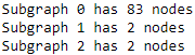
The results will tell you how big each of the connected components is. My results had one big subgraph of 83 users and the others have fewer users.
We can alter the threshold to alter the connected components. This is because a higher threshold has fewer edges connecting nodes, and therefore will have smaller connected components and more of them. We can see this by running the preceding code with a higher threshold:
G = create_graph( friends, 0.2 )

# We then use NetworkX to find the connected components in the graph
sub_graphs = nx.connected_component_subgraphs(G)

# To get a sense of the sizes of the graph,
# we can iterate over the groups and print out some basic information:
for i, sub_graph in enumerate( sub_graphs ):
    n_nodes = len( sub_graph.nodes() )
    print( 'Subgraph {0} has {1} nodes'.format(i, n_nodes) )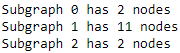
The preceding code gives us much smaller nodes and more of them. My largest cluster was broken into at least 3 parts and none of the clusters had more than 15 users. An example cluster is shown in the following figure, and the connections within this cluster are also shown. Note that, as it is a connected component, there were no edges from nodes in this component to other nodes in the graph (at least, with the threshold set at 0.2):
In a new cell, obtain the connected components and also the count of the connected components:
sub_graphs = nx.connected_component_subgraphs(G)
n_subgraphs = nx.number_connected_components(G)

n_subgraphs![]()
sub_graphs = nx.connected_component_subgraphs(G)
n_subgraphs = nx.number_connected_components(G) # n_subgraphs = 3

fig = plt.figure( figsize=(20, (n_subgraphs * 3)) )

for i, sub_graph in enumerate(sub_graphs):
    ax = fig.add_subplot(int(n_subgraphs / 3)+1, 3, i+1)
    ax.get_xaxis().set_visible(False)
    ax.get_yaxis().set_visible(False)
nx.draw(sub_graph, ax=ax) 
sub_graphs = nx.connected_component_subgraphs(G)
n_subgraphs = nx.number_connected_components(G) # n_subgraphs = 3

fig = plt.figure( figsize=(20, (n_subgraphs * 3)) )

for i, sub_graph in enumerate(sub_graphs):
    ax = fig.add_subplot(int(n_subgraphs / 3)+1, 3, i+1)
    ax.get_xaxis().set_visible(False)
    ax.get_yaxis().set_visible(False)
    pos = nx.spring_layout(G)
    nx.draw_networkx_nodes( G, pos, sub_graph.nodes(), ax=ax, node_size=500 )
    nx.draw_networkx_edges( G, pos, sub_graph.edges(), ax=ax)
The results visualize each connected component, giving us a sense of the number of nodes in each and also how connected they are.

If you are not seeing anything on your graphs, try rerunning the line:
sub_graphs = nx.connected_component_subgraphs(G)The sub_graphs object is a generator and is "consumed" after being used.
Optimizing criteria
Our algorithm for finding these connected components relies on the threshold parameter, which dictates whether edges are added to the graph or not. In turn, this directly dictates how many connected components we discover and how big they are. From here, we probably want to settle on some notion of which is the best threshold to use. This is a very subjective problem, and there is no definitive answer. This is a major problem with any cluster analysis task.
We can, however, determine what we think a good solution should look like and define a metric based on that idea. As a general rule, we usually want a solution where:
- • Samples in the same cluster (connected components) are highly similar to each other
- • Samples in different clusters are highly dissimilar to each other
The Silhouette Coefficient is a metric that quantifies these points.
Evaluation of clusters with silhouette coefficient: the silhouette coefficient is a measure of the compactness[kəmˈpæktnəs,ˈkɑːmpæktnəs]紧密度 and separation of the clusters. Higher values represent a better quality of cluster. The silhouette coefficient is higher for compact clusters that are well separated and lower for overlapping clusters. Silhouette coefficient values do change from -1 to +1, and the higher the value is, the better. Silhouette analysis can be used as a graphical tool to plot a measure of how tightly grouped the samples in the clusters are. To calculate the silhouette coefficient of a single sample in our dataset, we can apply the following three steps:
- Calculate the cluster cohesion[koʊˈhiːʒn]内聚度
 (is the mean intra cluster distance) as the average distance between a sample
  and all other points in the same cluster.
 - Calculate the cluster separation分离度
 from the next closest cluster(depicts mean nearest cluster distance) as the average distance between the sample and all samples in the nearest cluster.
 - Calculate the silhouette
 as the difference between cluster cohesion and separation divided by the greater of the two, as shown here:
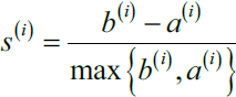 : the silhouette coefficient==
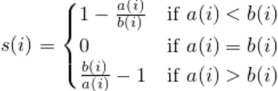
The silhouette coefficient is bounded in the range -1 to 1:
- a coefficient close to +1 means that the instance is well inside its own cluster and far from other clusters, while
- a coefficient close to 0 means that it is close to a cluster boundary, and
- finally a coefficient close to -1 means that the instance may have been assigned to the wrong cluster).
Based on the preceding formula, we can see that the silhouette coefficient is 0 if the cluster separation and cohesion are equal (![]() =
=![]() ). Furthermore, we get close to an ideal silhouette coefficient of 1 if
). Furthermore, we get close to an ideal silhouette coefficient of 1 if ![]() >>
>>![]() , since
, since ![]() quantifies how dissimilar a sample is to other clusters, and
quantifies how dissimilar a sample is to other clusters, and ![]() tells us how similar it is to the other samples in its own cluster, respectively.
tells us how similar it is to the other samples in its own cluster, respectively.
To compute the overall Silhouette Coefficient, we take the mean of the Silhouettes for each sample. A clustering that provides a Silhouette Coefficient close to the maximum of 1 has clusters that have samples all similar to each other, and these clusters are very spread apart. Values near 0 indicate that the clusters all overlap and there is little distinction between clusters. Values close to the minimum of -1 indicate that samples are probably in the wrong cluster, that is, they would be better off in other clusters.
Using this metric, we want to find a solution (that is, a value for the threshold) that maximizes the Silhouette Coefficient by altering the threshold parameter. To do that, we create a function that takes the threshold as a parameter and computes the Silhouette Coefficient.
We then pass this into the optimize module of SciPy, which contains the minimize function that is used to find the minimum value of a function by altering one of the parameters. While we are interested in maximizing the Silhouette Coefficient, SciPy doesn't have a maximize function. Instead, we minimize the inverse of the Silhouette (which is basically the same thing).
The scikit-learn library has a function for computing the Silhouette Coefficient, sklearn.metrics.silhouette_score; however, it doesn't fix the function format that is required by the SciPy minimize function. The minimize function requires the variable parameter to be first (in our case, the threshold value), and any arguments to be after it. In our case, we need to pass the friends dictionary as an argument in order to compute the graph. The code is as follows:
The Silhouette is also only defined if we have at least two connected components (in order to compute the inter-cluster distance, 2 <= nx.number_connected_components(G)), and at least one of these connected components has two members (to compute the intra-cluster distance, 2 <= nx.number_connected_components(G) < len(G.nodes() )-1 )). We test for these conditions and return our invalid problem score if it doesn't fit. The code is as follows:
However, the values are based on our weights, which are a similarity and not a distance. For a distance, higher values indicate more difference. We can convert from similarity to distance by subtracting the value from the maximum possible value, which for our weights was 1: X = 1-X
Now we have our distance matrix and labels, so we have all the information we need to compute the Silhouette Coefficient. We pass the metric as precomputed; otherwise, the matrix X will be considered a feature matrix, not a distance matrix (feature matrices are used by default nearly everywhere in scikit-learn). The code is as follows:
import numpy as np
from sklearn.metrics import silhouette_score

def compute_silhouette( threshold, friends ):
    # create the graph using the threshold parameter
    G = create_graph( friends, threshold=threshold )
    # check it has at least some nodes
    if len( G.nodes() ) < 2:
        return -99 # return a very poor score to indicate an invalid problem
                    # (Any valid solution will score higher than this)

    # extract the connected components
    sub_graphs = nx.connected_component_subgraphs(G)
                    # number_of_subgraphs
    if not ( 2 <= nx.number_connected_components(G) < len(G.nodes() )-1 ):
        return -99

    label_dict = {}
    for i, sub_graph in enumerate( sub_graphs ):
        for node in sub_graph.nodes():
            label_dict[node] = i
    # Then we iterate over the nodes in the graph to get the label for each node in order.
    # We need to do this two-step process, as
    # nodes are not clearly ordered within a graph
    # but they do maintain their order as long as no changes are made to the graph.
    # What this means is that, until we change the graph,
    # we can call .nodes() on the graph to get the same ordering. The code is as follows:
    labels = np.array([ label_dict[node]
                        for node in G.nodes()
                      ])
    # nx.to_scipy_sparse_matrix(G) : returns the graph in a matrix format,
    # the r_index and c_index of matrix is node position, value in each cell is weight, default 1
    X = nx.to_scipy_sparse_matrix(G).todense()
    X = 1-X
    return silhouette_score( X, labels, metric='precomputed' )
We have two forms of inversion happening here. The first is taking the inverse of the similarity to compute a distance function(X = 1-X); this is needed, as the Silhouette Coefficient only accepts distances. The second is the inverting of the Silhouette Coefficient score so that we can minimize with SciPy's optimize module.
def inverted_silhouette( threshold, friends ):
    return -compute_silhouette(threshold, friends)
The parameters are as follows:
- • invert(compute_silhouette): This is the function we are trying to minimize (remembering that we invert it to turn it into a loss function)
- • 0.01: This is an initial guess at a threshold that will minimize the function
- • options={'maxiter':20}: This dictates that only 20 iterations are to be performed (increasing this will probably get a better result, but will take longer to run)
- • method='nelder-mead': This is used to select the Nelder-Mead optimize routing (SciPy supports quite a number of different options)
- • args=(friends,): This passes the friends dictionary to the function that is being minimized
result = minimize(inverted_silhouette, 0.01, method='nelder-mead', args=(friends,), options={'maxiter':20, })
print(result) 
G = create_graph( friends, 0.008875 )

# We then use NetworkX to find the connected components in the graph
sub_graphs = nx.connected_component_subgraphs(G)

# To get a sense of the sizes of the graph,
# we can iterate over the groups and print out some basic information:
for i, sub_graph in enumerate( sub_graphs ):
    n_nodes = len( sub_graph.nodes() )
print( 'Subgraph {0} has {1} nodes'.format(i, n_nodes) )![]() try more data!!!
try more data!!!
Running this function, I got a threshold of 0.008875 that returns 2 components. The score returned by the minimize function was -0.0257. However, we must remember that we negated this value. This means our score was actually 0.0257. The value is positive, which indicates that the clusters tend to be more separated than not (a good thing). We could run other models and check whether it results in a better score, which means that the clusters are better separated.
We could use this result to recommend users—if a user is in a connected component, then we can recommend other users in that component. This recommendation follows our use of the Jaccard Similarity to find good connections between users, our use of connected components to split them up into clusters, and our use of the optimization technique to find the best model in this setting.
However, a large number of users may not be connected at all, so we will use a different algorithm to find clusters for them.
Summary
We created a graph of friends from a social network, in this case Twitter. We then examined how similar two users were, based on their friends. Users with more friends in common were considered more similar, although we normalize this by considering the overall number of friends they have. This is a commonly used way to infer knowledge (such as age or general topic of discussion) based on similar users. We can use this logic for recommending users to others—if they follow user X and user Y is similar to user X, they will probably like user Y. This is, in many ways, similar to our transaction-led similarity of previous chapters.
The aim of this analysis was to recommend users, and our use of cluster analysis allowed us to find clusters of similar users. To do this, we found connected components on a weighted graph we created based on this similarity metric. We used the NetworkX package for creating graphs, using our graphs, and finding these connected components.
We then used the Silhouette Coefficient, which is a metric that evaluates how good a clustering solution is. Higher scores indicate a better clustering, according to the concepts of intra-cluster and inter-cluster distance. SciPy's optimize module was used to find the solution that maximises this value.
In this chapter, we compared a few opposites too. Similarity is a measure between two objects, where higher values indicate more similarity between those objects. In contrast, distance is a measure where lower values indicate more similarity. Another contrast we saw was a loss function, where lower scores are considered better (that is, we lost less). Its opposite is the score function, where higher scores are considered better.
In the next chapter, we will see how to extract features from another new type of data: images. We will discuss how to use neural networks to identify numbers in images and develop a program to automatically beat CAPTCHA images.


 1万+
1万+


 被折叠的 条评论
为什么被折叠?
被折叠的 条评论
为什么被折叠?
 到【灌水乐园】发言


