m06_twitter U Naive Bayes_PermissionError [Errno 13]_NLP_bag词袋_Ngram_spaCy_pipeline_joblib_os创建进入子目录

     Text-based datasets contain a lot of information, whether they are books, historical documents, social media, e-mail, or any of the other ways we communicate via writing. Extracting features from text-based datasets and using them for classification is a difficult problem. There are, however, some common patterns for text mining.

     We look at disambiguating[ˌdɪsæmˈbɪɡjʊeɪtɪŋ]消除歧义 terms in social media using the Naive Bayes algorithm, which is a powerful and surprisingly simple algorithm. Naive Bayes takes a few shortcuts to properly compute the probabilities for classification, hence the term naive in the name. It can also be extended to other types of datasets quite easily and doesn't rely on numerical features. The model in this chapter is a baseline for text mining studies, as the process can work reasonably well for a variety of datasets.

We will cover the following topics in this chapter:

• • Downloading data from social network APIs
• • Transformers for text
• • Naive Bayes classifier
• • Using JSON for saving and loading datasets
• • The NLTK library for extracting features from text
• • The F-measure for evaluation

Disambiguation

     Text is often called an unstructured format. There is a lot of information there, but it is just there; no headings, no required format, loose syntax and other problems prohibit[prəˈhɪbɪt,proʊˈhɪbɪt]使不可能 the easy extraction of information from text. The data is also highly connected, with lots of mentions and cross-references—just not in a format that allows us to easily extract it!

     We can compare the information stored in a book with that stored in a large database to see the difference. In the book, there are characters, themes, places, and lots of information. However, the book needs to be read and, more importantly, interpreted to gain this information. The database sits on your server with column names and data types. All the information is there and the level of interpretation needed is quite low. Information about the data, such as its type or meaning is called metadata, and text lacks it. A book also contains some metadata in the form of a table of contents and index but the degree is significantly lower than that of a database.

     One of the problems is the term disambiguation. When a person uses the word bank, is this a financial message or an environmental message (such as river bank)? This type of disambiguation is quite easy in many circumstances for humans (although there are still troubles), but much harder for computers to do.

     In this chapter, we will look at disambiguating the use of the term Python on Twitter's stream. A message on Twitter is called a tweet and is limited to 140 characters(Tweets include lots of metadata, such as the time and date of posting, who posted it, and so on.). This means there is little room for context. There isn't much metadata available although hashtags“#” are often used to denote the topic of the tweet.

When people talk about Python, they could be talking about the following things:

• • The programming language Python
• • Monty Python, the classic comedy group
• • The snake Python蟒蛇
• • A make of shoe called Python

     There can be many other things called Python. The aim of our experiment is to take a tweet mentioning Python and determine whether it is talking about the programming language, based only on the content of the tweet.

     we are going to perform a data mining experiment consisting of the following steps:

• 1. Download a set of tweets from Twitter.
• 2. Manually classify them to create a dataset.
• 3. Save the dataset so that we can replicate our research.
• 4. Use the Naive Bayes classifier to create a classifier to perform term disambiguation.

Downloading data from a social network

     We are going to download a corpus of data from Twitter and use it to sort out剔除 spam from useful content. Twitter provides a robust API for collecting information from its servers and this API is free for small-scale usage. It is, however, subject to some conditions that you'll need to be aware of if you start using Twitter's data in a commercial setting.

     First, you'll need to sign up for a Twitter account (which is free). Go to http://twitter.com and register an account if you do not already have one.

     Next, you'll need to ensure that you only make a certain number of requests per minute. This limit is currently 15 requests per 15 minutes (it depends on the exact API). It can be tricky ensuring that you don't breach[briːtʃ]违反 this limit, so it is highly recommended that you use a library to talk to Twitter's API.

     If you are using your own code (that is making the web calls with your own code) to connect with a web-based API, ensure that you read the documentation about rate limiting their documentation and understand the limitations. In Python, you can use the time library to perform a pause between calls to ensure you do not breach the limit.

     You will need a key to access Twitter's data. Go to http://twitter.com and sign in to your account. When you are logged in, go to https://developer.twitter.com/en/apps and click on Create New App.Create a name and description for your app, along with a website address. If you don't have a website to use, insert a placeholder. Leave the Callback URL field blank for this app—we won't need it. Agree to the terms of use (if you do) and click on Create your Twitter application.

 >

 

==> API Key and Secret

 Access Token and Secret ==>

     Keep the resulting website open—you'll need the access keys that are on this page. Next, we need a library to talk to Twitter. There are many options; the one I like is simply called twitter, and is the official Twitter Python library.

     You can install twitter using pip3 install twitter (on the command line) if you are using pip to install your packages. At the time of writing, Anaconda does not include twitter, therefore you can't use conda to install it. If you are using another system or want to build from source, check the documentation at https://github.com/sixohsix/twitter

     Create a new Jupyter Notebook to download the data. We will create several notebooks in this chapter for various different purposes, so it might be a good idea to also create a folder to keep track of them. This first notebook, ch6_get_twitter, is specifically for downloading new Twitter data.

     First, we import the twitter library and set our authorization tokens. The consumer key, consumer secret will be available on the Keys and Access Tokens tab on your Twitter app's page. To get the access tokens, you'll need to click on the Create my access token button, which is on the same page. Enter the keys into the appropriate places in the following code:

import twitter

# API Key and Secret
consumer_key = 'HW5MoQ6BfFVZhhV5IahfhNQXV'
consumer_secret = 'ouzrDgvdZOpa7AFdcrYrRKezNWaTN5p08JeU9UdnOnnyNsl0KI'
# Access Token and Secret
access_token = '1441908129701138436-trVsSMGs518y9hvRS8dmMBrCXlzPsE'
access_token_secret = 'QasEX8VSD1oN1FwRQgNIIBcrh3alC8sVKiG3ofgOUD9JI'

authorization = twitter.OAuth( access_token, access_token_secret,
                               consumer_key, consumer_secret
                             )

     We are going to get our tweets from Twitter's search function. We will create a reader that connects to twitter using our authorization, and then use that reader to perform searches. In the Notebook, we set the filename where the tweets will be stored:

import os
output_filename = os.path.join(os.path.expanduser("~"), "data", "datasets", "twitter", "python_tweets.json")
print(output_filename)

import os

# PermissionError: [Errno 13] Permission denied: 'dataset/twitter/python_tweets.json'
#                  path = os.path.join( '/'.join(["dataset","twitter", "python_tweets.json"]) )
#                  since python_tweets.json is a folder after os.makedir(path) instead of a json file
# solution:
path = os.path.join( '/'.join(["dataset","twitter"]) )
if not os.path.exists( path ):
    os.mkdir(path)
output_filename = path + "/python_tweets.json"
output_filename

 PermissionError: [Errno 13]

 

     Next, create an object that can read from Twitter. We create this object with our authorization object that we set up earlier:

t = twitter.Twitter( auth=authorization )

     We then open our output file for writing. We open it for appending—this allows us to rerun the script to obtain more tweets. We then use our Twitter connection to perform a search for the word Python. We only want the statuses that are returned for our dataset. This code takes the tweet, uses the json library to create a string representation using the dumps function, and then writes it to the file. It then creates a blank line under the tweet so that we can easily distinguish where one tweet starts and ends in our file:

import json

n_output = 0

# https://www.w3schools.com/python/ref_func_open.asp
# "a" - Append - Opens a file for appending, creates the file if it does not exist
with open( output_filename, 'a' ) as output_file:
    # https://developer.twitter.com/en/docs/twitter-api/v1/tweets/search/api-reference/get-search-tweets
    search_results = t.search.tweets( q='python', count=100 )['statuses']
    for tweet in search_results:
        if 'text' in tweet:
            output_file.write( json.dumps(tweet) )
            output_file.write('\n\n')
            n_output +=1

print('Saved {} entries'.format(n_output) )

https://developer.twitter.com/en/docs/twitter-api/v1/tweets/search/api-reference/get-search-tweets
     In the preceding loop, we also perform a check to see whether there is text in the tweet or not. Not all of the objects returned by twitter will be actual tweets (for example, some responses will be actions to delete tweets). The key difference is the inclusion of text as a key, which we test for消息对象与其他对象的关键不同在于消息对象中含有键“text”，这也正是我们用if语句进行检测的. 

Running this for a few minutes will result in 100 tweets being added to the output file.

     You can keep rerunning this script to add more tweets to your dataset, keeping in mind that you may get some duplicates in the output file if you rerun it too fast (that is, before Twitter gets new tweets to return!).For our initial experiment, 100 tweets will be enough, but you will probably want to come back and rerun this code to get that up to about 1000.

Loading and classifying the dataset

     After we have collected a set of tweets (our dataset), we need labels to perform classification. We are going to label the dataset by setting up a form in a Jupyter Notebook to allow us to enter the labels. We do this by loading the tweets we collected in the previous section, iterating over them and providing (manually) a classification on whether they refer to Python the programming language or not.

     The dataset we have stored is nearly, but not quite, in a JSON format. JSON is a format for data that doesn't impose much structure on the contents, just on the syntax. The idea behind JSON is that the data is in a format directly readable in JavaScript (hence the name, JavaScript Object Notation). JSON defines basic objects such as numbers, strings, lists, and dictionaries, making it a good format for storing datasets, if they contain data that isn't numerical. If your dataset is fully numerical, you would save space and time using a matrix-based format like in NumPy.

     A key difference between our dataset and real JSON is that we included newlines between tweets. The reason for this was to allow us to easily append new tweets (the actual JSON format doesn't allow this easily). Our format is a JSON representation of a tweet, followed by a newline, followed by the next tweet, and so on.

     To parse it, we can use the json library but we will have to first split the file by newlines to get the actual tweet objects themselves. Set up a new Jupyter Notebook, I called mine ch6_label_twitter. Within it, we will first load the data from our input filename by iterating over the file, storing tweets as we loop. The code below does a basic check that there is actual text in the tweet. If it does, we use the json library to load the tweet and then we add it to a list:

import json
import os

# path = os.path.join( '/'.join(["dataset","twitter"]) )
# if not os.path.exists( path ):
#     os.mkdir(path)
input_filename = path + "/python_tweets.json"
labels_filename = path + '/python_classes.json'

tweet_list = []
with open( input_filename ) as inputfile:
    for line in inputfile:
        if len( line.strip() ) == 0:
            continue
        # else: use json.loads (which loads a JSON object from a string)   
        tweet_list.append( json.loads(line) )

     We are now interested in classifying whether an item is relevant to us or not (in this case, relevant means refers to the programming language Python). We will use the IPython Notebook's ability to embed HTML and talk between JavaScript and Python to create a viewer of tweets to allow us to easily and quickly classify the tweets as spam or not.

     The code will present a new tweet to the user (you) and ask for a label: is it relevant or not? It will then store the input and present the next tweet to be labeled.

     As stated, we will use the json library, so import that too:

import json

     We create a list that will store the tweets we received from the file. These labels will be stored whether or not the given tweet refers to the programming language Python, and it will allow our classifier to learn how to differentiate between meanings.

tweet_list = []

     We then iterate over each line in the file. We aren't interested in lines with no information (they separate the tweets for us), so check if the length of the line (minus any whitespace characters) is zero. If it is, ignore it and move to the next line. Otherwise, load the tweet using json.loads (which loads a JSON object from a string) and add it to our list of tweets. The code is as follows:

import json
import os

# path = os.path.join( '/'.join(["dataset","twitter"]) )
# if not os.path.exists( path ):
#     os.mkdir(path)
input_filename = path + "/python_tweets.json"
labels_filename = path + '/python_classes.json'

tweet_list = []
with open( input_filename ) as inputfile:
    for line in inputfile:
        if len( line.strip() ) == 0:
            continue
        # else: use json.loads (which loads a JSON object from a string)   
        tweet_list.append( json.loads(line) )

tweet_list[0]

 ... ... 

   We are now interested in classifying whether an item is relevant to us or not (in this case, relevant means refers to the programming language Python). We will use the IPython Notebook's ability to embed HTML and talk between JavaScript and Python to create a viewer of tweets to allow us to easily and quickly classify the tweets as spam or not.

     The code will present a new tweet to the user (you) and ask for a label: is it relevant or not? It will then store the input and present the next tweet to be labeled.

     First, we create a list for storing the labels. These labels will be stored whether or not the given tweet refers to the programming language Python, and it will allow our classifier to learn how to differentiate between meanings.

     We also check if we have any labels already and load them. This helps if you need to close the notebook down midway through labeling. This code will load the labels from where you left off. It is generally a good idea to consider how to save at midpoints for tasks like this. Nothing hurts quite like losing an hour of work because your computer crashed before you saved the labels! The code is as follows:

labels = []
if os.path.exists( labels_filename ):
    with open( labels_filename ) as inputfile:
        labels = json.load( inputfile )

     Next, we create a simple function that will return the next tweet that needs to be labeled. We can work out which is the next tweet by finding the first one that hasn't yet been labeled. The code is as follows:

def get_next_tweet():
    return tweet_list[ len(labels) ]['text']

get_next_tweet()

     The next step in our experiment is to collect information from the user (you!) on which tweets are referring to Python (the programming language) and which are not. As of yet, there is not a good, straightforward way to get interactive feedback with pure Python in IPython Notebooks. For this reason, we will use some JavaScript and HTML to get this input from the user.

     Next we create some JavaScript in the IPython Notebook to run our input. Notebooks allow us to use magic functions to embed HTML and JavaScript (among other things) directly into the Notebook itself. Start a new cell with the following line at the top:

%%html

     At the end of that function, we call the load_next_tweet function. This function loads the next tweet to be labeled. It runs on the same principle; we load the IPython kernel and give it a command to execute (calling the get_next_tweet function we defined earlier).

     However, in this case we want to get the result. This is a little more difficult. We need to define a callback, which is a function that is called when the data is returned. The format for defining callback is outside the scope of this book. If you are interested in more advanced JavaScript/Python integration, consult the IPython documentation.

    function load_next_tweet(){
        var code_input = "get_next_tweet()";
        var kernel = IPython.notebook.kernel;
        var callbacks = { "iopub" : { "output" : handle_output} }
        kernel.execute( code_input, callbacks, { silent : false } )
    }

 code_input ==> kernel.execute ==> callbacks(handle_output)

###############################
Messaging in Jupyter — jupyter_client 7.0.3 documentation

1. IOPub: this socket is the ‘broadcast channel’ where the kernel publishes all side effects (stdout, stderr, debugging events etc.) as well as the requests coming from any client over the shell socket and its own requests on the stdin socket. There are a number of actions in Python which generate side effects: print() writes to sys.stdout, errors generate tracebacks, etc. Additionally, in a multi-client scenario, we want all frontends to be able to know what each other has sent to the kernel (this can be useful in collaborative scenarios, for example). This socket allows both side effects and the information about communications taking place with one client over the shell channel to be made available to all clients in a uniform manner.

2. General Message Format

   1. The content dict is the body of the message. Its structure is dictated by the msg_type field in the header, described in detail for each message below.

###############################

     The callback function is called handle_output, which we will define now. This function gets called when the Python function that kernel.execute calls returns a value. As before, the full format of this is outside the scope of this book. However, for our purposes the result is returned as data of the type text/plain, which we extract and show in the #tweet_text div of the form we are going to create in the next cell. The code is as follows:

    function handle_output( out ){
        // "out" is the object passed to the callback from the kernel execution
        console.log( out ); // to display text(here is out) on the console
        
        // the result is returned as data of the type text/plain,
        // which we extract and show in the <div id="tweet_text"> of the form
        // we are going to create in the next cell
        var res = out.content.data["text/plain"];
        
        
        // pass a string(here is value of res) to html(), that string will be used for the 
        // plain-text or HTML-formatted text content of the element(here is <div id="tweet_text">
        $("div#tweet_text").html(res);
    }

     We are going to use a different magic function now, %%html. Unsurprisingly, this magic function allows us to directly embed HTML into our Notebook. In a new cell, start with this line:

     Our form will have a div that shows the next tweet to be labeled, which we will give the ID #tweet_text. We also create a textbox to enable us to capture key presses (otherwise, the Notebook will capture them and JavaScript won't do anything). This allows us to use the keyboard to set labels of 1 or 0, which is faster than using the mouse to click buttons—given that we will need to label at least 100 tweets.

     For this cell, we will be coding in HTML and a little JavaScript. First, define a div element to store our current tweet to be labeled. I've also added some instructions for using this form. Then, create the #tweet_text div that will store the text of the next tweet to be labeled. As stated before, we need to create a textbox to be able to capture key presses. The code is as follows:

%%html
<div name = "tweetbox">
    Instruction: Click in text box. Enter a 1 if the tweet is relevant, enter 0 otherwise.</br>
    Tweet: <div id="tweet_text" value="text"></div></br>
    <input type="text" id="capture"></input</br>
</div>

     We create the JavaScript for capturing the key presses. This has to be defined after creating the form, as the #tweet_text div doesn't exist until the above code runs. We use the JQuery library (which IPython is already using, so we don't need to include the JavaScript file) to add a function that is called when key presses are made on the #capture textbox we defined. However, keep in mind that this is a %%html cell and not a JavaScript cell, so we need to enclose this JavaScript in the <script> tags. 

     We are only interested in key presses if the user presses the 0 or the 1, in which case the relevant label is added. We can determine which key was pressed by the ASCII value stored in e.which. If the user presses 0 or 1, we append the label and clear out the textbox. The code is as follows:

    $("input#capture").keypress( function(e){
                                    console.log(e);
                                    if (e.which == 48){
                                        // 0 pressed and 0 : ASCII code==48
                                        $( "input#capture" ).val(""); // clear out the textbox
                                        set_label(0);
                                    }else if (e.which == 49){
                                        // 1 pressed and 1 : ASCII code=49
                                        $( "input#capture" ).val(""); // clear out the textbox
                                        set_label(1);
                                    }else{
                                        $( "input#capture" ).val(""); // clear out the textbox
                                    }
 
                                 }
                               );

     After you enter a classification number, it will call and display the next tweet, set_label function, press Enter, the text box will be cleared (if the input is not 1 or 0, the text box will be cleared again), and then display the next tweet. So if the Enter key is not pressed, the text box will not be cleared(since textbox has not capture the Enter key presses), even if the current classification number has been used, and the next tweet to be classified has been displayed.

All other key presses are ignored.

     we will define in JavaScript shows how easy it is to talk to your Python code from JavaScript in IPython Notebooks. This function, if called, will add a label to the labels array (which is in python code). To do this, we load the IPython kernel as a JavaScript object and give it a Python command to execute. The code is as follows:

    function set_label(label){
        var kernel = IPython.notebook.kernel;
        kernel.execute( "labels.append(" + label + ")" );
        load_next_tweet();
    }

     As a last bit of JavaScript for this chapter (I promise), we call the load_next_tweet() function. This will set the first tweet to be labeled and then close off the JavaScript. The code is as follows:

%%html
<div name = "tweetbox">
    Instruction: Click in text box. Enter a 1 if the tweet is relevant, enter 0 otherwise.</br>
    Tweet: <div id="tweet_text" value="text"></div></br>
    <input type="text" id="capture"></input</br>
</div>


<script>
    function set_label(label){
        var kernel = IPython.notebook.kernel;
        kernel.execute( "labels.append(" + label + ")" );
        load_next_tweet();
    }
    
    function handle_output( out ){
        // "out" is the object passed to the callback from the kernel execution
        console.log( out ); // to display text(here is out) on the console
        
        // the result is returned as data of the type text/plain,
        // which we extract and show in the <div id="tweet_text"> of the form
        // we are going to create in the next cell
        var res = out.content.data["text/plain"];
        
        
        // pass a string(here is value of res) to html(), that string will be used for the 
        // plain-text or HTML-formatted text content of the element(here is <div id="tweet_text">
        $("div#tweet_text").html(res);
    }

    function load_next_tweet(){
        var code_input = "get_next_tweet()";
        var kernel = IPython.notebook.kernel;
        var callbacks = { "iopub" : { "output" : handle_output} };
        kernel.execute( code_input, callbacks, { silent : false } );
    }
                                                           
    $("input#capture").keypress( function(e){
                                    console.log(e);
                                    if (e.which == 48){
                                        // 0 pressed and 0 : ASCII code==48
                                        $( "input#capture" ).val(""); // clear out the textbox
                                        set_label(0);
                                    }else if (e.which == 49){
                                        // 1 pressed and 1 : ASCII code=49
                                        $( "input#capture" ).val(""); // clear out the textbox
                                        set_label(1);
                                    }else{
                                        $( "input#capture" ).val(""); // clear out the textbox
                                    }
 
                                 }
                               );

load_next_tweet();                                                                    
</script>

     After you run this cell, you will get an HTML textbox, alongside the first tweet's text. Click in the textbox and enter 1 if it is relevant to our goal (in this case, it means is the tweet related to the programming language Python) and a 0 if it is not. After you do this, the next tweet will load. Then press Enter key to clear out the textbox. Next, Enter the label(1 or 0) for the current tweet. This continues until the tweets run out

     Originally I only had 100 tweets, so when the marked category exceeds 100, the tweet shown above will always be the last one. But the labels stored in the labels list will exceed, which is where the current code is not perfect.

len(labels)

     When you finish all of this, simply save the labels to the output filename we defined earlier for the class values:

# labels_filename = path + '/python_classes.json'
with open(labels_filename, 'w') as outf:
    json.dump(labels[:100], outf) # OR json.dump(labels, outf)

 

     You can call the preceding code even if you haven't finished. Any labeling you have done to that point will be saved. Running this Notebook again will pick up where you left off and you can keep labeling your tweets.

     This might take a while to do this! If you have a lot of tweets in your dataset, you'll need to classify all of them. If you are pushed for time, you can download the same dataset I used, which contains classifications.

Creating a replicable dataset from Twitter

     In data mining, there are lots of variables. These aren't just in the data mining algorithms—they also appear in the data collection, environment, and many other factors. Being able to replicate复制 your results is important as it enables you to verify or improve upon your results.

     Getting 80 percent accuracy on one dataset with algorithm X, and 90 percent accuracy on another dataset with algorithm Y doesn't mean that Y is better. We need to be able to test on the same dataset in the same conditions to be able to properly compare.

     On running the preceding code, you will get a different dataset to the one I created and used. The main reasons are that Twitter will return different search results for you than me based on the time you performed the search. Even after that, your labeling of tweets might be different from what I do. While there are obvious examples where a given tweet relates to the python programming language, there will always be gray areas where the labeling isn't obvious. One tough gray area I ran into was tweets in non-English languages that I couldn't read. In this specific instance, there are options in Twitter's API for setting the language, but even these aren't going to be perfect.

     Due to these factors, it is difficult to replicate experiments on databases that are extracted from social media, and Twitter is no exception. Twitter explicitly disallows sharing datasets directly.

     One solution to this is to share tweet IDs only, which you can share freely. In this section, we will first create a tweet ID dataset that we can freely share. Then, we will see how to download the original tweets from this file to recreate the original dataset.

     First, we save the replicable dataset of tweet IDs. Creating another new IPython Notebook, first set up the filenames. This is done in the same way we did labeling but there is a new filename where we can store the replicable dataset. The code is as follows:

import os

path = os.path.join( '/'.join(["dataset","twitter"]) )
input_filename = path + "/python_tweets.json"
labels_filename = path + '/python_classes.json'
replicable_dataset = path + '/python_replicable_dataset.json'

We load the tweets and labels as we did in the previous notebook:

import json

tweets = []

with open( input_filename ) as inputFile:
    for line in inputFile:
        if len( line.strip() ) == 0:
            continue
        tweets.append( json.loads(line) )

if os.path.exists( labels_filename ):
    with open( labels_filename ) as inputFile:
        labels = json.load( inputFile )

tweets[0]

     Now we create a dataset by looping over both the tweets and labels at the same time and saving those in a list:

dataset = [ (tweet['id'], label) 
            for label, tweet in zip( labels, tweets)
          ]
dataset[:3]

 

Finally, we save the results in our file:

len( dataset ), len( tweets), len( labels )

     Now that we have the tweet IDs and labels saved, we can recreate the original dataset. If you are looking to recreate the dataset I used for this chapter, it can be found in the code bundle that comes with this book

with open( replicable_dataset, 'w' ) as outputFile:
    json.dump( dataset, outputFile )

 ​

##### recreate the dataset

import os

# PermissionError: [Errno 13] Permission denied: 'dataset/twitter/python_tweets.json'
#                  path = os.path.join( '/'.join(["dataset","twitter", "python_tweets.json"]) )
#                  since python_tweets.json is a folder after os.makedir(path) instead of a json file
# solution:
path = os.path.join( '/'.join(["dataset","twitter", "recreate"]) )
if not os.path.exists( path ):
    os.mkdir(path)
tweet_filename = path + "/python_tweets.json"
labels_filename = path + '/replicable_python_classes.json'
replicable_dataset = path + '/replicable_dataset.json' # id, label

 ​

 https://raw.githubusercontent.com/PacktPublishing/Learning-Data-Mining-with-Python/master/Chapter%206/replicable_dataset.json

new create a file and named it replicable_dataset, then copy data online and paste to it. 

[[546508356979281920, 1], [546508223466192896, 0], [546508177227796480, 0], [546508108789338112, 1], [546508007865987072, 1], [546507926903742464, 0], [546507853666975745, 1], [546507847249313792, 1], [546507772171649024, 0], [546507705234784257, 0], [546507685643161600, 1], [546507676742864896, 0], [546507632073138176, 0], [546507342867865600, 0], [546507150290190336, 0], [546506674945929216, 1], [546506607107264512, 0], [546506601914716162, 1], [546506550459002880, 0], [546506540820463616, 1], [546506425455747073, 1], [546506373328953345, 1], [546506358485295104, 1], [546506256056205312, 0], [546506117627789313, 1], [546506093044973568, 1], [546506092021559297, 1], [546505992901390336, 1], [546505983535886336, 1], [546505978355515392, 1], [546505978225491968, 1], [546505977965473792, 1], [546505967760715777, 0], [546505818699755520, 1], [546505736680120320, 1], [546505687753175040, 1], [546505677834027008, 0], [546505677405822978, 1], [546505672947691520, 0], [546505611022581761, 1], [546505474603229184, 0], [546505391308169217, 1], [546505358093860867, 1], [546505355308855296, 1], [546505336979734528, 0], [546505320127012864, 1], [546505197795561473, 0], [546505168598994944, 0], [546504988009037824, 0], [546504851727712256, 0], [546504823903100928, 1], [546504725592416256, 0], [546504705606971392, 1], [546504676267413505, 1], [546504659519549441, 0], [546504656914903040, 1], [546504593543561218, 0], [546504493991333888, 1], [546504411279659009, 0], [546504368040972288, 1], [546504303939039232, 0], [546504253448404993, 1], [546504234829492224, 0], [546504161207271425, 0], [546504160485863424, 0], [546504108249997312, 0], [546504106609623040, 0], [546504104797696000, 0], [546504103317495808, 0], [546504098586308608, 0], [546504097646780416, 0], [546504095952306176, 1], [546503915240312833, 1], [546503912388190208, 1], [546503909586399232, 1], [546503906788786178, 1], [546503903387209729, 1], [546503898442117120, 1], [546503891555065856, 0], [546503889835413505, 1], [546503854171226113, 0], [546503817953419264, 0], [546503791282237440, 1], [546503670422978561, 0], [546503536914497537, 1], [546503505813311489, 0], [546503505804922881, 0], [546503256214888448, 1], [546503249872687104, 0], [546503151134965760, 0], [546503047816691713, 0], [546502991163846656, 0], [546502959081984000, 1], [546502898675617793, 0], [546502893726351360, 0], [546502892967174144, 0], [546502862474604544, 1], [546502763354783744, 0], [546502761727393792, 0], [546502744748470273, 0], [546599833742880768, 1], [546599774720630784, 1], [546599604653801472, 1], [546599603437842432, 0], [546599578313576448, 1], [546599576300318721, 1], [546599414689574912, 1], [546599259223498753, 0], [546599196162158592, 0], [546599056315670528, 1], [546599055095132160, 1], [546598995284348928, 0], [546598985419345921, 1], [546598982755971073, 1], [546598952364433408, 1], [546598943975419904, 1], [546598936283078657, 1], [546598811292815360, 1], [546598808654581760, 1], [546598802975506433, 1], [546598799150301184, 1], [546598779550707712, 0], [546598739524485120, 1], [546598714886742016, 1], [546598695630671872, 1], [546598619655049217, 1], [546598607668117504, 1], [546598593013248000, 1], [546598584322629632, 1], [546598549236891649, 1], [546598524352495616, 0], [546598497579835393, 1], [546598451170258944, 1], [546598450578862080, 0], [546598437177667584, 1], [546598344034762752, 0], [546598040334000128, 1], [546597988269703170, 0], [546597962160570368, 1], [546597913468862465, 1], [546597696921141248, 1], [546597617690349570, 1], [546597567895965696, 1], [546597465344851968, 0], [546597460907274240, 0], [546597445942411265, 0], [546597406130057216, 1], [546597211342008321, 0], [546597157445578753, 0], [546597121122512897, 0], [546597060661628928, 0], [546597040168255488, 1], [546597037311946752, 1], [546597033419616256, 1], [546596986044940288, 1], [546596939836719104, 1], [546596885117411329, 0], [546596830411104256, 0], [546596736404582400, 0], [546596711947202561, 0], [546596573090549760, 0], [546596486624985088, 0], [546596464638828544, 1], [546596463774818304, 1], [546596367477391360, 0], [546596353548111872, 0], [546596342236061696, 0], [546596314470162432, 0], [546596307154915328, 0], [546596294186127362, 0], [546596269012291584, 0], [546596253614632960, 0], [546596197863927810, 0], [546596188598706177, 0], [546596072164818944, 1], [546595958864482304, 1], [546595953646374913, 1], [546595885506121728, 0], [546595831487295488, 1], [546595823140626432, 1], [546595822771531779, 0], [546595821320278017, 1], [546595804387885056, 0], [546595759731511296, 1], [546595551564009472, 1], [546595540847562752, 1], [546595437789331457, 0], [546595362879070208, 1], [546595317031116800, 1], [546595141440786432, 0], [546595062659178498, 0], [546595062067765249, 0], [546595060075462656, 0], [546595048763035648, 0], [546595043218571264, 1], [546594904369946624, 0], [546594789471186944, 1], [546594687436324865, 0], [546594627667505153, 0], [546594612354097152, 0]]

​
Then load the tweet IDs from the file using JSON:

import json

with open( replicable_dataset ) as inputFile:
    tweet_ids = json.load( inputFile )

     Saving the labels is very easy. We just iterate through this dataset and extract the IDs. We could do this quite easily with just two lines of code (open file and save tweets). However, we can't guarantee that we will get all the tweets we are after (for example, some may have been changed to private since collecting the dataset) and therefore the labels will be incorrectly indexed against the data.

     As an example, I tried to recreate the dataset just one day after collecting them and already two of the tweets were missing (they might be deleted or made private by the user). For this reason, it is important to only print out the labels that we need. To do this, we first create an empty actual labels list to store the labels for tweets that we actually recover from twitter, and then create a dictionary mapping the tweet IDs to the labels.

The code is as follows:

actual_labels = []
label_mapping = dict( tweet_ids ) # e.g. 546508356979281920: 1 # id:label

     Next, we are going to create a twitter server to collect all of these tweets. This is going to take a little longer. Import the twitter library that we used before, creating an authorization token and using that to create the twitter object:

import twitter

# API Key and Secret
consumer_key = 'HW5MoQ6BfFVZhhV5IahfhNQXV'
consumer_secret = 'ouzrDgvdZOpa7AFdcrYrRKezNWaTN5p08JeU9UdnOnnyNsl0KI'
# Access Token and Secret
access_token = '1441908129701138436-trVsSMGs518y9hvRS8dmMBrCXlzPsE'
access_token_secret = 'QasEX8VSD1oN1FwRQgNIIBcrh3alC8sVKiG3ofgOUD9JI'

authorization = twitter.OAuth( access_token, access_token_secret,
                               consumer_key, consumer_secret
                             )

t = twitter.Twitter(auth=authorization)

     The following code will loop through our tweets in groups of 100, join together the id values, and get the tweet information for each of them.

     Besides, we perform a statuses/lookup API call, which is defined by Twitter. We pass our list of IDs (which we turned into a string) into the API call in order to have those tweets returned to us

all_ids = [tweet_id for tweet_id, label in tweet_ids]
tweet_temp=[]

with open(tweet_filename, 'a') as output_file:
    # We can lookup 100 tweets at a time, which saves time in asking twitter for them
    for start_index in range(0, len(all_ids), 100):
        id_string = ",".join(str(i) for i in all_ids[start_index:start_index+100])
        search_results = t.statuses.lookup( _id=id_string ) ######################
        for tweet in search_results:
            if 'text' in tweet:
                # Valid tweet - save to file
                output_file.write(json.dumps(tweet))
                output_file.write("\n\n")
                tweet_temp.append(tweet)
                actual_labels.append(label_mapping[tweet['id']])

     In this code, we then check each tweet to see if it is a valid tweet and then save it to our file if it is. Our final step is to save our resulting labels:

with open(labels_filename, 'w') as outf:
    json.dump(actual_labels, outf)

len(actual_labels), len(all_ids), len(tweet_temp)

​

Combine old and new data sets

labels_filename = os.path.join('dataset/twitter/python_classes.json')
label_list = []

with open( labels_filename ) as inputFile:
    label_list = json.load( inputFile )

len(label_list)

  I just labeled 100 tweets

tweet_filename = os.path.join('dataset/twitter/python_tweets.json')
tweet_list = []

import json
 
with open( tweet_filename ) as inputFile:
    for line in inputFile:
        if len( line.strip() ) == 0:
            continue
        tweet_list.append( json.loads(line) )

len( tweet_list[:100] )

 

 Old data set

labels_filename = os.path.join('dataset/twitter/recreate/replicable_python_classes.json')
label_replicable = []

with open( labels_filename ) as inputFile:
    label_replicable = json.load( inputFile )

len(label_replicable)

 

tweet_filename = os.path.join('dataset/twitter/recreate/python_tweets.json')
tweet_replicable = []

with open( tweet_filename ) as inputFile:
    for line in inputFile:
        if len( line.strip() ) == 0:
            continue
        tweet_replicable.append( json.loads(line) )

len(tweet_replicable)

 

 Append the new tweets to the end

with open(tweet_filename, 'a') as output_file:
    for tweet in tweet_list[:100]:# since I just labeled 100 tweets
        output_file.write( json.dumps(tweet) )
        output_file.write("\n\n")

tweet_filename = os.path.join('dataset/twitter/recreate/python_tweets.json')
tweet_replicable = []

with open( tweet_filename ) as inputFile:
    for line in inputFile:
        if len( line.strip() ) == 0:
            continue
        tweet_replicable.append( json.loads(line) )
len(tweet_replicable)  

 
 since there is a list in replicable_python_classes.json, so we can't not use an append operation

combined_label_list=label_replicable +label_list

with open(labels_filename, 'w') as output_file:
    output_file.write( json.dumps(combined_label_list) )

labels_filename = os.path.join('dataset/twitter/recreate/replicable_python_classes.json')
label_replicable = []

with open( labels_filename ) as inputFile:
    label_replicable = json.load( inputFile )
len(label_replicable)

 

Text transformers

Now that we have our dataset, how are we going to perform data mining on it?

      Text-based datasets include books, essays, websites, manuscripts, programming code, and other forms of written expression. All of the algorithms we have seen so far deal with numerical or categorical features, so how do we convert our text into a format that the algorithm can deal with?

     There are a number of measurements that could be taken. For instance, average word and average sentence length are used to predict the readability of a document. However, there are lots of feature types such as word occurrence which we will now investigate.

Bag-of-words

cp8_Sentiment_urlretrieve_pyprind_tarfile_bag词袋_walk目录_regex_verbose_N-gram_Hash_colab_verbose_文本向量化_Linli522362242的专栏-CSDN博客

n3_knn breastCancer NaiveBayesLikelihood_voter_manhat_Euclid_Minkow_空值?_SBS特征选取_Laplace_zip_NLP_spam_Linli522362242的专栏-CSDN博客

13_Load Preproc4_[..., np.newaxis]_ExitStack_walk_file操作_timeit_regex_feature vector embed_Text Toke_Linli522362242的专栏-CSDN博客

     One of the simplest but highly effective models is to simply count each word in the dataset. We create a matrix, where each row represents a document in our dataset and each column represents a word. The value of the cell is the frequency of that word in the document.

Here's an excerpt from The Lord of the Rings指环王, J.R.R. Tolkien:

Three Rings for the Elven-kings under the sky,
Seven for the Dwarf-lords in halls of stone,
Nine for Mortal Men, doomed to die,
One for the Dark Lord on his dark throne
In the Land of Mordor where the Shadows lie.
One Ring to rule them all, One Ring to find them,
One Ring to bring them all and in the darkness bind them.
In the Land of Mordor where the Shadows lie.
                                       - J.R.R. Tolkien's epigraph to The Lord of The Rings

     The word the appears 9 times in this quote, while the words in, for, to, and one each appear 4 times. The word ring appears 3 times, as does the word of.

     We can create a dataset from this, choosing a subset of words and counting the frequency:
​
     We can use the counter class to do a simple count for a given string. When counting words, it is normal to convert all letters to lowercase, which we do when creating the string. The code is as follows:

# Converting words into lowercase
s = """Three Rings for the Elven-kings under the sky,
Seven for the Dwarf-lords in halls of stone,
Nine for Mortal Men, doomed to die,
One for the Dark Lord on his dark throne
In the Land of Mordor where the Shadows lie.
One Ring to rule them all, One Ring to find them,
One Ring to bring them all and in the darkness bind them.
In the Land of Mordor where the Shadows lie.""".lower()

s

​

import string
                  # inner join for recreating an new paragraph including "\n"
texts = " ".join( "".join( [" " if ch in string.punctuation else ch
                                for ch in s
                           ]# Removal of punctuations or replace all punctuations with blank
                         ).split() # return a word_array or remove "\n"
                ) # outer join for recreating an new paragraph excluding "\n"

texts

​

import nltk

 # step2                    # Return a sentence-tokenized copy of text # In fact, it’s not needed here, just to show
tokens = [ word for sent in nltk.sent_tokenize( texts )
                    for word in nltk.word_tokenize(sent)
        ]                   # Return a tokenized copy of text
tokens[:9]

 ​

     Stop words are the words that repeat so many times in literature and yet are not a differentiator in the explanatory power of sentences.

     Stop-words are simply those words that are extremely common in all sorts of texts and probably bear no (or only a little) useful information that can be used to distinguish between different classes of documents. Examples of stopwords are is, and, has, and so on. Removing stop-words can be useful if we are working with raw or normalized term frequencies rather than tf-idfs(可以用于减轻特征向量中这些频繁出现的单词的权重。), which are already downweighting frequently occurring words.

     For example: I, me, you, this, that, the, and so on, which needs to be removed before further processing.

     stop words are the words that do not carry much weight in understanding the sentence; they are used for connecting words, and so on. We have removed them with the following line of code:

from nltk.corpus import stopwords

stopwds = stopwords.words('english')
tokens = [token for token in tokens
                     if token not in stopwds
         ]# step4 Stop word removal
tokens

​

     Stemming process stems the words to its respective root words. Example of stemming is bringing down running to run or runs to run. By doing stemming we reduce duplicates and improve the accuracy of the model.

# tokens = [ word for word in tokens if len(word)>=3 ] # step5 of length at least three

from nltk.stem import PorterStemmer

stemmer = PorterStemmer()
tokens = [ stemmer.stem(word) for word in tokens ]   # step 6 Stemming of words

tokens[:9]

​

from collections import Counter

c = Counter( tokens )
c

​ 

c.most_common(6)

​​​

compare to:

from collections import Counter

c = Counter( texts.split() ) # or s.split()
c.most_common(5)

​

     Printing c.most_common(5) gives the list of the top five most frequently occurring words. Ties are not handled well as only five are given and a very large number of words all share a tie for 2nd place竟然有4个词并列第二.

     The bag-of-words model has three major types, with many variations and alterations.

• The first is to use the raw frequencies原始频率, as shown in the preceding example. This has the same drawback as any non-normalised data - words with high variance due to high overall values (such as) the overshadow lower frequency (and therefore lower-variance) words, even though the presence of the word the rarely has much importance是当文档长度差异明显时，词频差距会非常大.
• The second model is to use the normalized frequency, where each document's sum equals 1. This is a much better solution as the length of the document doesn't matter as much, but it still means words like the overshadow lower frequency words. The third type is to simply use binary features—a value is 1 if it occurs, and 0 otherwise这种做法优势明显，它规避了文档长度对词频的影响. We will use binary representation in this chapter.
• Another (arguably more popular) method for performing normalization is called term frequency-inverse document frequency (tf-idf). In this weighting scheme, term counts are first normalized to frequencies and then divided by the number of documents in which it appears in the corpus. We will use tf-idf in Chapter 10, Clustering News Articles. OR
  n3_knn breastCancer NaiveBayesLikelihood_voter_manhat_Euclid_Minkow_空值?_SBS特征选取_Laplace_zip_NLP_spam_Linli522362242的专栏-CSDN博客
  cp8_Sentiment_urlretrieve_pyprind_tarfile_bag词袋_walk目录_regex_verbose_N-gram_Hash_colab_verbose_文本向量化_Linli522362242的专栏-CSDN博客

     There are a number of libraries for working with text data in Python. We will use a major one, called Natural Language ToolKit (NLTK). The scikit-learn library also has the CountVectorizer class that performs a similar action, and it is recommended you take a look at it (we will use it in Chapter 9, Authorship Attribution). However the NLTK version has more options for word tokenization. If you are doing natural language processing in python, NLTK is a great library to use. 

N-grams

     One variation on the standard bag-of-words model is called the n-gram model. An n-grams model addresses the deficiency of context in the bag-of-words model. With a bag-of-words model, only individual words are counted by themselves. This means that common word pairs, such as United States, lose meaning they have in the sentence because they are treated as individual words.

     There are algorithms that can read a sentence, parse it into a tree-like structure, and use this to create very accurate representations of the meaning behind words. Unfortunately, these algorithms are computationally expensive. This makes it difficult to apply them to large datasets.

     To compensate for these issues of context and complexity, the n-grams model fits into the middle ground. It has more context than the bag-of-words model, while only being slightly more expensive computationally.

     An n-gram is a subsequence of n consecutive, overlapping, tokens. In this experiment, we use word n-grams, which are n-grams of word-tokens. They are counted the same way as a bag-of-words, with the n-grams forming a word that is put in the bag. The value of a cell in this dataset is the frequency that a particular n-gram appears in the given document.

     They are counted the same way, with the n-grams forming a word that is put in the bag. The value of a cell in this dataset is the frequency that a particular n-gram appears in the given document.

     The value of n is a parameter. For English, setting it to between 2 to 5 is a good start, although some applications call for higher values. Higher values for n result in sparse datasets, as when n increases it is less likely to have the same n-gram appear across multiple documents. Having n=1 results in simply the bag-of-words model.

As an example, for n=3, we extract the first few n-grams in the following quote:

Always look on the bright side of life.

     The first n-gram (of size 3) is Always look on, the second is look on the, the third is on the bright. As you can see, the n-grams overlap and cover three words each. Word n-grams have advantages over using single words. This simple concept introduces some context to word use by considering its local environment, without a large overhead of understanding the language computationally.

     A disadvantage of using n-grams is that the matrix becomes even sparser—word n-grams are unlikely to appear twice (especially in tweets and other short documents!). Specifically for social media and other short documents, word n-grams are unlikely to appear in too many different tweets, unless it is a retweet. However, in larger documents, word n-grams are quite effective for many applications. Another form of n-gram for text documents is that of a character ngram. That said, you'll see shortly that word n-grams are quite effective in practice.

     Rather than using sets of words, we simply use sets of characters (although character n-grams have lots of options for how they are computed!). This type of model can help identify words that are misspelled, as well as providing other benefits to classification. We will test character n-grams in this chapter and see them again in Chapter 9, Authorship Attribution.

Other text features

     There are other features that can be extracted too. These include syntactic[sɪnˈtæktɪk]语法的 features, such as the usage of particular words in sentences. Part-of-speech tags词性标签 are also popular for data mining applications that need to understand meaning in text. Such feature types won't be covered in this book. If you are interested in learning more, I recommend Python 3 Text Processing with NLTK 3 Cookbook, Jacob Perkins, Packt publication.

     There are a number of libraries for working with text data in Python. The most commonly known one is called the Natural Language ToolKit (NLTK). The scikitlearn library also has the CountVectorizer class that performs a similar action, and it is recommended you take a look at it (we will use it in Chapter 9, Authorship Attribution). NLTK has more features for word tokenization and part of speech tagging (that is identifying which words are nouns, verbs and so on).

     The library we are going to use is called spaCy. It is designed from the ground up to be fast and reliable for natural language processing. Its less-well-known than NLTK, but is rapidly growing in popularity. It also simplifies some of the decisions, but has a slightly more difficult syntax to use, compared to NLTK.

     For production systems, I recommend using spaCy, which is faster than NLTK. NLTK was built for teaching, while spaCy was built for production. They have different syntaxes, meaning it can be difficult to port code from one library to another. If you aren't looking into experimenting with different types of natural language parsers, I recommend using spaCy.

Naive Bayes

     Naive Bayes is a probabilistic model that is, unsurprisingly, built upon a naive interpretation of Bayesian statistics. Despite the naive aspect, the method performs very well in a large number of contexts. Because of the naive aspect, it works quite quickly. It can be used for classification of many different feature types and formats, but we will focus on one in this chapter: binary features in the bag-ofwords model.

Understanding Bayes' theorem

     For most of us, when we were taught statistics, we started from a frequentist approach从频率论者. In this approach, we assume the data comes from some distribution and we aim to determine what the parameters are for that distribution. However, those parameters are (perhaps incorrectly) assumed to be fixed. We use our model to describe the data, even testing to ensure the data fits our model.

     Bayesian statistics instead model how people (at least, non-frequentist statisticians) actually reason. We have some data, and we use that data to update our model about how likely something is to occur. In Bayesian statistics, we use the data to describe the model rather than using a model and confirming it with data (as per the frequentist approach).

     It should be noted that frequentist statistics and Bayesian statistics ask and answer slightly different questions. A direct comparison is not always correct.

     Bayes' theorem computes the value of P(A|B). That is, knowing that B has occurred, what is the probability of event A occurring. In most cases, B is an observed event such as it rained yesterday, and A is a prediction it will rain today. For data mining, B is usually we observed this sample and A is does the sample belong to this class (the class prediction). We will see how to use Bayes' theorem for data mining in the next section.

The equation for Bayes' theorem is given as follows: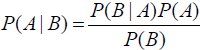
​
     As an example, we want to determine the probability that an e-mail containing the word drugs is spam (as we believe that such a tweet may be a pharmaceutical spam).

     A, in this context, is the probability that this tweet is spam. We can compute P(A), called the prior belief directly from a training data by computing the percentage of tweets in our dataset that are spam. If our dataset contains 30 spam messages for every 100 e-mails, P(A) is 30/100 or 0.3.

     B, in this context, is this tweet contains the word drugs. Likewise, we can compute P(B) by computing the percentage of tweets in our dataset containing the word drugs. If 10 e-mails in every 100 of our training dataset contain the word drugs, P(B) is 10/100 or 0.1. Note that we don't care if the e-mail is spam or not when computing this value.

     P(B|A) is the probability that an e-mail contains the word drugs if it is spam. This is also easy to compute from our training dataset. We look through our training set for spam e-mails and compute the percentage of them that contain the word drugs. Of our 30 spam e-mails, if 6 contain the word drugs, then P(B|A) is calculated as 6/30 or 0.2.

     From here, we use Bayes' theorem to compute P(A|B), which is the probability that a tweet containing the word drugs is spam. Using the previous equation, we see the result is 0.6. This indicates that if an e-mail has the word drugs in it, there is a 60 percent chance that it is spam.

     Note the empirical nature of the preceding example—we use evidence directly from our training dataset, not from some preconceived distribution. In contrast, a frequentist view of this would rely on us creating a distribution of the probability of words in tweets to compute similar equations.

Naive Bayes algorithm

     Looking back at our Bayes' theorem equation, we can use it to compute the probability that a given sample belongs to a given class. This allows the equation to be used as a classification algorithm.

     With C as a given class and D as a sample in our dataset, we create the elements necessary for Bayes' theorem, and subsequently Naive Bayes. Naive Bayes is a classification algorithm that utilizes Bayes' theorem to compute the probability that a new data sample belongs to a particular class.

     P(D) is the probability of a given data sample. It can be difficult to compute this, as the sample is a complex interaction between different features, but luckily it is constant across all classes. Therefore, we don't need to compute it at all, as all we do in the final step is compare relative values.

     P(C|D) is the probability of the data point belonging to the class. This could also be difficult to compute due to the different features. However, this is where we introduce the naive part of the Naive Bayes algorithm. We naively assume that each feature is independent of each other. Rather than computing the full probability of P(C|D), we compute the probability of each feature D1, D2, D3, ... and so on. Then, we just multiply them together:
P(C|D) = P(C|D1) x P(C|D2) x P(C|D3) x ... x P(C|Dn)
     Each of these values is relatively easy to compute with binary features; we simply compute the percentage of times it is equal in our sample dataset.

     In contrast, if we were to perform a non-naive Bayes version of this part, we would need to compute the correlations between different features for each class. Such computation is infeasible at best, and nearly impossible without vast amounts of data or adequate language analysis models.

     From here, the algorithm is straightforward. We compute P(C|D) for each possible class, ignoring the P(D) term. Then we choose the class with the highest probability. As the P(D) term is consistent across each of the classes, ignoring it has no impact on the final prediction.

n3_knn breastCancer NaiveBayesLikelihood_voter_manhat_Euclid_Minkow_空值?_SBS特征选取_Laplace_zip_NLP_spam_Linli522362242的专栏-CSDN博客

How it works

     As an example, suppose we have the following (binary) feature values from a sample in our dataset: [0, 0, 0, 1].

     Our training dataset contains two classes with 75 percent of samples belonging to the class 0(P(C=0)=0.75), and 25 percent belonging to the class 1(P(C=1)). The likelihood of the feature values for each class are as follows:

For class 0: [0.3, 0.4, 0.4, 0.7] <== [ P(D1=1|C=0) , P(D2|C=0) , P(D3|C=0) , P(D4|C=0) ]
For class 1: [0.7, 0.3, 0.4, 0.9]

These values are to be interpreted as: for feature 1, it is a 1 in 30 percent of cases for class 0.

     We can now compute the probability that this sample should belong to the class 0. P(C=0) = 0.75 which is the probability that the class is 0.

P(D) isn't needed for the Naive Bayes algorithm. Let's take a look at the calculation:

P(C=0|D) = P(D1=1|C=0) x P(D2=0|C=0) x P(D3=0|C=0) x P(D4=1|C=0)
                = 0.3 x 0.6 x 0.6 x 0.7
                = 0.0756

     The second and third values are 0.6, because the value of that feature in the sample was 0. The listed probabilities are for values of 1 for each feature. Therefore, the probability of a 0 is its inverse: P(0) = 1 – P(1).

     Now, we can compute the probability of the data point belonging to this class. An important point to note is that we haven't computed P(D), so this isn't a real probability. However, it is good enough to compare against the same value for the probability of the class 1. Let's take a look at the calculation:

P(C=0|D) = P(C=0) P(D|C=0) without / ( P(D1=1) x P(D2=0) x P(D3=0) x P(D4=1) )
                = 0.75 * 0.0756
                = 0.0567

Now, we compute the same values for the class 1:

P(C=1) = 0.25 = 1 - 0.75

P(D) isn't needed for naive Bayes. Let's take a look at the calculation:

P(C=1|D) = P(D1=1|C=1) x P(D2=1|C=1) x P(D3=1|C=1) x P(D4=1|C=1)
                = 0.7 x 0.7 x 0.6 x 0.9
                = 0.2646
P(C=1|D) = P(C=1) P(D|C=1) without / ( P(D1=1) x P(D2=1) x P(D3=1) x P(D4=1) )
                = 0.25 * 0.2646
                = 0.06615

     Normally, P(C=0|D) + P(C=1|D) should equal to 1. After all, those are the only two possible options! However, the probabilities are not 1 due to the fact we haven't included the computation of P(D) in our equations here.

     The data point should be classified as belonging to the class 1. You may have guessed this while going through the equations anyway; however, you may have been a bit surprised that the final decision was so close. After all, the probabilities in computing P(C=0|D) were much, much higher for the class 1. This is because we introduced a prior belief that most samples generally belong to the class 0.

     If the classes had been equal sizes, the resulting probabilities would be much different. Try it yourself by changing both P(C=0) and P(C=1) to 0.5 for equal class sizes and computing the result again.

Applying of Naive Bayes

     We will now create a pipeline that takes a tweet and determines whether it is relevant or not, based only on the content of that tweet.

     To perform the word extraction, we will be using the spaCy, a library that contains a large number of tools for performing analysis on natural language. We will use spaCy in future chapters as well.

     To get spaCy on your computer, use pip to install the package: pip install spacy
If that doesn't work, see the spaCy installation instructions at https://spacy.io/ for information specific to your platform.

pip install spacy && python -m spacy download en

We are going to create a pipeline to extract the word features and classify the tweets using Naive Bayes. Our pipeline has the following steps:

• Transform the original text documents into a dictionary of counts using spaCy's word tokenization.
• Transform those dictionaries into a vector matrix using the DictVectorizer transformer in scikit-learn. This is necessary to enable the Naive Bayes classifier to read the feature values extracted in the first step.
• Train the Naive Bayes classifier, as we have seen in previous chapters.

     We will need to create another Notebook (last one for the chapter!) called ch6_classify_twitter for performing the classification.

Extracting word counts

     We are going to use spaCy to extract our word counts. We still want to use it in a pipeline, but spaCy doesn't conform to our transformer interface. We will need to create a basic transformer to do this to obtain both fit and transform methods, enabling us to use this in a pipeline.

     First, set up the transformer class. We don't need to fit anything in this class, as this transformer simply extracts the words in the document. Therefore, our fit is an empty function, except that it returns self which is necessary for transformer objects to conform to the scikit-learn API.

     Our transform is a little more complicated. We want to extract each word from each document and record True if it was discovered. We are only using the binary features here—True if in the document, False otherwise. If we wanted to use the frequency we would set up counting dictionaries, as we have done in several of the past chapters.

English · spaCy Models Documentation

13_Load Preproc4_[..., np.newaxis]_ExitStack_walk_file操作_timeit_regex_feature vector embed_Text Toke_Linli522362242的专栏-CSDN博客

import spacy
from sklearn.base import TransformerMixin

# Create a spaCy parser
nlp = spacy.load('en_core_web_sm')

class BagOfWords( TransformerMixin ):
    def fit( self, X, y=None ):
        return self
    
    def transform( self, X ):
        results = [] # a list of dictionaries
        for document in X:
            row = {}
            for word in list( nlp(document) ):
                if len( word.text.strip() ):
                    row[word.text] = True
            results.append( row )
        return results

     The result is a list of dictionaries, where the first dictionary is the list of words in the first tweet, and so on. Each dictionary has a word as key and the value True to indicate this word was discovered. Any word not in the dictionary will be assumed to have not occurred in the tweet. Explicitly stating that a word's occurrence is False will also work, but will take up needless space to store.

Converting dictionaries to a matrix

     The next step converts the dictionaries built as per the previous step into a matrix that can be used with a classifier. This step is made quite simple through the DictVectorizer transformer that is provided as part of scikit-learn.

     The DictVectorizer class simply takes a list of dictionaries and converts them into a matrix. The features in this matrix are the keys in each of the dictionaries, and the values correspond to the occurrence of those features in each sample. Dictionaries are easy to create in code, but many data algorithm implementations prefer matrices. This makes DictVectorizer a very useful class.

     In our dataset, each dictionary has words as keys and only occurs if the word actually occurs in the tweet. Therefore, our matrix will have each word as a feature and a value of True in the cell if the word occurred in the tweet.

To use DictVectorizer, simply import it using the following command:

from sklearn.feature_extraction import DictVectorizer

Training the Naive Bayes classifier

     Finally, we need to set up a classifier and we are using Naive Bayes for this chapter. As our dataset contains only binary features, we use the BernoulliNB classifier that is designed for binary features. As a classifier, it is very easy to use. As with DictVectorizer, we simply import it and add it to our pipeline:

from sklearn.naive_bayes import BernoulliNB

     Now comes the moment to put all of these pieces together. In our Jupyter Notebook, set the filenames and load the dataset and classes as we have done before. Set the filenames for both the tweets themselves (not the IDs!) and the labels that we assigned to them. The code is as follows:

import os

# PermissionError: [Errno 13] Permission denied: 'dataset/twitter/python_tweets.json'
#                  path = os.path.join( '/'.join(["dataset","twitter", "python_tweets.json"]) )
#                  since python_tweets.json is a folder after os.makedir(path) instead of a json file
# solution:
path = os.path.join( '/'.join(["dataset","twitter", "recreate"]) )
if not os.path.exists( path ):
    os.mkdir(path)
tweet_filename = path + "/python_tweets.json"
labels_filename = path + '/replicable_python_classes.json'

     Load the tweets themselves. We are only interested in the content of the tweets, so we extract the text value and store only that. The code is as follows:

import json

tweets = []
with open( input_filename ) as inputFile:
    for line in inputFile:
        if len( line.strip() ) == 0:
            continue
        tweets.append( json.loads(line)['text'] )

with open( labels_filename ) as inputFile:
    labels = json.load( inputFile )
    
# Ensure only classified tweets are loaded
tweets = tweets[:len(labels)]
assert len(tweets) == len(labels)

len(tweets), len(labels)

     Now, create a pipeline putting together the components from before. Our pipeline has three parts:

• 1. The NLTKBOW transformer we created.
• 2. A DictVectorizer transformer.
• 3. A BernoulliNB classifier.

The code is as follows:

from sklearn.pipeline import Pipeline

pipeline = Pipeline( [( 'bag-of-words', BagOfWords() ),
                      ( 'vectorizer', DictVectorizer() ),
                      ( 'naive-bayes', BernoulliNB() )
                     ] )

     We can nearly run our pipeline now, which we will do with cross_val_score as we have done many times before. Before we perform the data mining, we will introduce a better evaluation metric than the accuracy metric we used before. As we will see, the use of accuracy is not adequate for datasets when the number of samples in each class is different.

Evaluation using the F1-score

     When choosing an evaluation metric, it is always important to consider cases where that evaluation metric is not useful. Accuracy is a good evaluation metric in many cases, as it is easy to understand and simple to compute. However, it can be easily faked. In other words, in many cases, you can create algorithms that have a high accuracy but have a poor utility.

     While our dataset of tweets (typically, your results may vary) contains about 50 percent programming-related and 50 percent nonprogramming, many datasets aren't as balanced as this.

     As an example, an e-mail spam filter may expect to see more than 80 percent of incoming e-mails be spam. A spam filter that simply labels everything as spam is quite useless; however, it will obtain an accuracy of 80 percent!

     To get around this problem, we can use other evaluation metrics. One of the most commonly employed is called an f1-score (also called f-score, f-measure, or one of many other variations on this term).

     The F1-score is defined on a per-class basis and is based on two concepts: the precision and recall. The precision is the percentage of all the samples that were predicted as belonging to a specific class, that were actually from that class. The recall is the percentage of samples in the dataset that are in a class and actually labeled as belonging to that class.

n2_Tree ML Models_HR data_Chi-square_SAMME_AdaBoost_GradientBoosting_XGBoost_class weight_Ensemble_Linli522362242的专栏-CSDN博客

03_Classification_2_regex_confusion matrix_.reshape([-1])_score(average=“macro“)_interpolation.shift_Linli522362242的专栏-CSDN博客

• Accuracy = (TP+TN)/(TP+FP+FN+TN) = (844 + 78)/(844+9+98+78) = 0.896
  Accuracy answers the following question: How many instances did we correctly label out of all the instances?
• Precision = TP/(TP+FP) # True predicted/ (True predicted + False predicted)  = 78/(78+9)=0.896
  Precision answers the following: How many of those who we labeled as target class(Attrition) are actually target class(Attrition=Yes)?
• Recall (aka Sensitivity) = TP/(TP+FN) = 78/(78+98) = 0.443
  Recall answers the following question: Of all the instances who are target class(Attrition=Yes), how many of those we correctly predict?
• F1 Score = 2*(Recall*Precision) / (Recall+Precision) = 2*(0.443*0.896)/(0.443+0.896)=0.593
  F1 Score considers both precision and recall.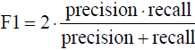

     In the case of our application, we could compute the value for both classes (python-programming and not python-programming).

     Our precision computation becomes the question: "of all the tweets that were predicted as being relevant, what percentage were actually relevant?"

     Likewise, the recall becomes the question: "of all the relevant tweets in the data set, how many were predicted as being relevant?"

     After you compute both the precision and recall, the f1-score is the harmonic mean of the precision and recall:

     To use the f1-score in scikit-learn methods, simply set the scoring parameter to f1. By default, this will return the f1-score of the class with label 1. Running the code on our dataset, we simply use the following line of code:

from sklearn.model_selection import cross_val_score

scores = cross_val_score( pipeline, tweets, labels, scoring='f1' )# cv=5 : default 5-fold

import numpy as np

print( 'Score: {:.3f}'.format( np.mean(scores) ) )

     The result is 0.532, which means we can accurately determine if a tweet using Python relates to the programing language nearly 53 percent of the time. This is using a dataset with only 104 tweets in it.

# Create a spaCy parser
nlp = spacy.load('en_core_web_sm')

class BagOfWords( TransformerMixin ):
    def fit( self, X, y=None ):
        return self
    
    def transform( self, X ):
        results = [] # a list of dictionaries
        for document in X:
            row = {}
            texts = " ".join( "".join( [" " if ch in string.punctuation else ch
                                                for ch in document
                                       ]# Removal of punctuations or replace all punctuations with blank
                                     ).split() # return a word_array or remove "\n"
                            ) # outer join for recreating an new paragraph excluding "\n"
            
            # step2                    # Return a sentence-tokenized copy of text # In fact, it’s not needed here, just to show
            tokens = [ word for sent in nltk.sent_tokenize( texts )
                                for word in nltk.word_tokenize(sent)
                     ]                   # Return a tokenized copy of text
            
#             stopwds = stopwords.words('english')
#             tokens = [token for token in tokens
#                                  if token not in stopwds
#                      ]# step4 Stop word removal
#             #stemmer = PorterStemmer()
#             tokens = [ stemmer.stem(word) for word in tokens ]   # step 6 Stemming of words
                       
            for word in tokens:
                    row[word] = True
            results.append( row )
        return results

from sklearn.model_selection import cross_val_score
from sklearn.pipeline import Pipeline

pipeline = Pipeline( [( 'bag-of-words', BagOfWords() ),
                      ( 'vectorizer', DictVectorizer() ),
                      ( 'naive-bayes', BernoulliNB() )
                     ] )

scores = cross_val_score( pipeline, tweets, labels, scoring='f1' )# cv=5 : default 5-fold

import numpy as np

print( 'Score: {:.3f}'.format( np.mean(scores) ) )

112tweets==>  Proved: Sometimes it’s not good to use the library directly 

212tweets==> 

     Go back and collect more data and you will find that the results increase! Keep in mind that your dataset may differ, and therefore your results would too.

More data usually means a better accuracy, but it is not guaranteed!

Getting useful features from models

     One question you may ask is, what are the best features for determining if a tweet is relevant or not? We can extract this information from our Naive Bayes model and find out which features are the best individually, according to Naive Bayes.

     First, we fit a new model. While the cross_val_score gives us a score across different folds of cross-validated testing data, it doesn't easily give us the trained models themselves. To do this, we simply fit our pipeline with the tweets, creating a new model. The code is as follows:

model = pipeline.fit( tweets, labels )

     Note that we aren't really evaluating the model here, so we don't need to be as careful with the training/testing split. However, before you put these features into practice, you should evaluate on a separate test split. We skip over that here for the sake of clarity.

     pipeline gives you access to the individual steps through the named_steps attribute and the name of the step (we defined these names ourselves when we created the pipeline object itself). For instance, we can get the Naive Bayes model:

nb = model.named_steps['naive-bayes']
feature_probabilities = nb.feature_log_prob_

feature_probabilities.shape

use 112 tweets <==2: binary ==> 0 : not exist; 1:exist  ==>use 212 tweets 

     From this model, we can extract the probabilities for each word. These are stored as log probabilities, which is simply log(P(A|f)), where f is a given feature.

     The reason these are stored as log probabilities is because the actual values are very low. For instance, the first value is -3.486, which correlates to a probability under 0.03 percent. Logarithm probabilities are used in computation involving small probabilities like this as they stop underflow errors where very small values are just rounded to zeros. Given that all of the probabilities are multiplied together, a single value of 0 will result in the whole answer always being 0! Regardless, the relationship between values is still the same; the higher the value, the more useful that feature is.

     We can get the most useful features by sorting the array of logarithm probabilities. We want descending order, so we simply negate the values first. The code is as follows:

top_features = np.argsort( -nb.feature_log_prob_[1])[:50] # return the feature indice

     The preceding code will just give us the indices and not the actual feature values. This isn't very useful, so we will map the feature's indices to the actual values. The key is the DictVectorizer step of the pipeline, which created the matrices for us. Luckily this also records the mapping, allowing us to find the feature names that correlate to different columns. We can extract the features from that part of the pipeline:

dv = model.named_steps['vectorizer']

     From here, we can print out the names of the top features by looking them up in the feature_names_ attribute of DictVectorizer. Enter the following lines into a new cell and run it to print out a list of the top features:

for i, feature_index in enumerate(top_features):
    print(i, dv.feature_names_[feature_index], #########
             np.exp( feature_probabilities[1][feature_index] )
         )

     The first few features include : RT, and even Python. These are likely to be noise (although the use of a colon is not very common outside programming, if you not removing punctuation, then your result may appear), based on the data we collected. Collecting more data is critical to smoothing out these issues. Looking through the list though, we get a number of more obvious programming features:

use 112tweets                                                      use 212tweets
==>
     There are some others too that refer to Python in a work context, and therefore might be referring to the programming language (although freelance snake handlers may also use similar terms, they are less common on Twitter). 

That last one is usually in the format: "We're looking for a candidate for this job".

     Looking through these features gives us quite a few benefits. We could train people to recognize these tweets, look for commonalities (which give insight into a topic), or even get rid of features that make no sense. For example, the word RT appears quite high in this list; however, this is a common Twitter phrase for retweet (that is, forwarding on someone else's tweet). An expert could decide to remove this word from the list, making the classifier less prone to the noise we introduced by having a small dataset.

Create a subdirectory and enter

import joblib
path = os.path.join( '/'.join(["models","twitter"]) )
# 'models/twitter'
if not os.path.exists( path ):
    for p in path.split('/'):
        deeper_path = os.path.join( os.getcwd(), p )
        print(deeper_path)
        if not os.path.exists(deeper_path):
            os.mkdir(deeper_path)
            os.chdir(deeper_path)
        else:
            os.chdir(deeper_path)
            continue
else:
    os.chdir(path)
# tweet_filename = path + "/python_tweets.json"
# labels_filename = path + '/replicable_python_classes.json'
os.getcwd()

 

output_model_filename = "python_context.pkl"
output_model_filename

 

joblib.dump( model, output_model_filename )

 

Summary

     In this chapter, we looked at text mining—how to extract features from text, how to use those features, and ways of extending those features. In doing this, we looked at putting a tweet in context—was this tweet mentioning python referring to the programming language? We downloaded data from a web-based API, getting tweets from the popular microblogging website Twitter. This gave us a dataset that we labeled using a form we built directly in the Jupyter Notebook.

     We also looked at reproducibility of experiments. While Twitter doesn't allow you to send copies of your data to others, it allows you to send the tweet's IDs. Using this, we created code that saved the IDs and recreated most of the original dataset. Not all tweets were returned; some had been deleted in the time since the ID list was created and the dataset was reproduced.

     We used a Naive Bayes classifier to perform our text classification. This is built upon the Bayes' theorem that uses data to update the model, unlike the frequentist method that often starts with the model first. This allows the model to incorporate and update new data, and incorporate a prior belief. In addition, the naive part allows to easily compute the frequencies without dealing with complex correlations between features.

     The features we extracted were word occurrences—did this word occur in this tweet? This model is called bag-of-words. While this discards information about where a word was used, it still achieves a high accuracy on many datasets. This entire pipeline of using the bag-of-words model with Naive Bayes is quite robust. You will find that it can achieve quite good scores on most text-based tasks. It is a great baseline for you, before trying more advanced models. As another advantage, the Naive Bayes classifier doesn't have any parameters that need to be set (although there are some if you wish to do some tinkering).

     To extend the work we did in this chapter, first start by collecting more data. You'll need to manually classify these as well, but you'll find some similarities between tweets that might make it easier. For example, there is a field of study called Locality Sensitive Hashes, that determines whether two tweets are similar. Two similar tweets are likely about the same topic. Another method for extending the research is to consider how you would build a model that incorporates the twitter user's history into the equation - in other words, if the user often tweets about python-as-a-programming-language, then they are more likely to be using python in a future tweet.

     In the next chapter, we will look at extracting features from another type of data, graphs, in order to make recommendations on who to follow on social media.