凸优化——判断问题是否为凸问题及转换技巧

提示：文章写完后，目录可以自动生成，如何生成可参考右边的帮助文档

---

前言（Preface）

注意：本文与《Convex Optimization》的Convex/Concave Function定义相同，但与同济大学《高等数学》的定义相反.

---

凸问题（Convex Problem）

凸问题的一般形式：
$$\begin{array}{rl}\min & f(x)\\ \text{s.t. }& h_i(x)=0,\forall i=1,...,n\\ & g_i(x)\le 0,\forall j=1,...,m\end{array}$$ 其中，目标函数$f(x)$是凸函数，等式约束$h_i(x)$为仿射，不等式约束$g_i(x)$为凸函数。

---

凸集（Convex Set）

定义

一个集合$C\subseteq {\mathbb{R}}^n$为凸集，如果满足任意$x,y\in C$有
$$tx+(1-t)y\in C,\forall 0\le t\le 1.$$

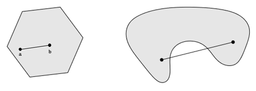
从几何的角度来看，任一两点在凸集内有连续的线段连接。例如下图中，图一成立，而图二不成立。

---

仿射函数（Affine Function）

定义（Definition）

从${\mathbb{R}}^n$到${\mathbb{R}}^m$的映射：$x\to Ax+b$，称为反射变换（Affine Transform）或仿射映射（Affine Map），其中$A$是一个$m\times n$矩阵，$b$是一个$m$维向量。当$m=1$时，称上述仿射变换称为仿射函数（Affine Function）。

一般形式：$$f(\mathbf{x})=\mathbf{A}\mathbf{x}+\mathbf{b}，$$其中，$\mathbf{A}$是一个$m\times k$矩阵，$x$是一个$k$向量，$b$是一个$m$向量，实际反映从$k$维到$m$维的空间映射关系。

若$f$是一个矢性（值）函数，若它可以表示为：$$f({\mathbf{x}}_1,...,{\mathbf{x}}_n)={\mathbf{A}}_1{\mathbf{x}}_1+{\mathbf{A}}_2{\mathbf{x}}_2+...+{\mathbf{A}}_n{\mathbf{x}}_n\mathbf{b}，$$ 其中，${\mathbf{A}}_i$可以是一个标量or矩阵，则称$f$是仿射函数。

充要条件（Necessary and Sufficient Condition）

$f[p{x}_1+(1-p)y_1,p{x}_2+(1-p)y_2,\dots ,p{x}_n+(1-p)y_n]\equiv pf(x_1,x_2,\dots ,x_n)+(1-p)f(y_1,y_2,\dots ,y_n)$

Comparison with Linear Function

当仿射函数中的$\mathbf{b}$中的元素全为零，即，截距为零，则称为线性函数（Linear Function）。

---

凸函数（Convex Function）

Definition of Convex Functions

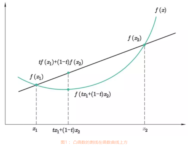
凸函数（一元）（Convex Function）：对于一元函数$f(x)$，如果对于任意$t\in [0,1]$，满足$f\left(t{x}_1+(1-t)x_2\right)\le tf(x_1)+(1-t)f(x_2)$，则称$f(x)$为凸函数（Convex Function）。

严格凸函数（一元）（Strictly Convex Function）：$\forall t\in (0,1)$，满足$f\left(t{x}_1+(1-t)x_2\right)<tf(x_1)+(1-t)f(x_2)$，则称$f(x)$为严格凸函数。注意：与凸函数相比，少了等号。

若从几何的角度来看，凸函数的割线在函数曲线的上方，线段上的点$(t{x}_1+(1-t)x_2,tf(x_1)+(1-t)f(x_2))$始终大于下方的点$\left(t{x}_1+(1-t)x_2,f\left(t{x}_1+(1-t)x_2\right)\right)$。

在数据科学的模型求解中，如果优化的目标函数是凸函数，则局部极小值就是全局最小值。

---

Judgement for Convex Functions (凸函数的判断)

A. General Methods for Convex Proof （凸证明的常用方法）

3.1.3 First-order conditions（一阶条件）

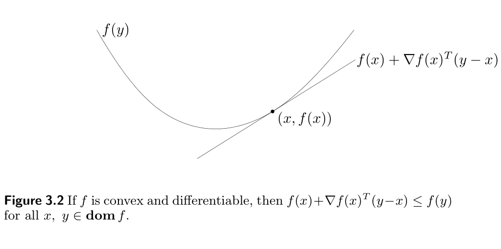
Suppose $f$ is differentiable (i.e., its gradient $\nabla f$ exists at each point in $\mathbf{d}\mathbf{o}\mathbf{m}f$, which is open). Then $f$ is convex, if and only if $\mathbf{d}\mathbf{o}\mathbf{m}f$ is convex and $$f(y)\ge f(x)+\nabla f(x{)}^T(y-x)(3.2)$$ holds for all $x,y\in \mathbf{d}\mathbf{o}\mathbf{m}f$.

Remarkable properties of convex functions and convex optimization problems

• The affine function of $y$ given by $f(x)+\nabla f(x{)}^T(y-x)$ is, of course, the first-order Taylor approximation of $f$ near $x$.
• The inequality $(3.2)$ states that for a convex function, the first-order Taylor approximation is in fact a global underestimator of the function.
• Conversely, if the first-order Taylor approximation of a function is always a global underestimator of the function, then the function is convex.

The inequality $(3.2)$ shows that from local information about a convex function (i.e., its value and derivative at a point) we can derive global information (i.e., a global underestimator of it).

This is perhaps the most important propoerty of convex functions, and explains some of the remarkable propoerties of convex functions and convex optimization problems.

As one simple example, the inequality $(3.2)$ shows that if $\nabla f(x)=0$, then for all $y\in \mathbf{d}\mathbf{o}\mathbf{m}f,$ $f(y)\ge f(x)$, i.e., $x$ is a global minimizer of the function $f$.

• Strict convexity can also be characterized by a first-order condition: $f$ is strictly convex if and only if $\mathbf{d}\mathbf{o}\mathbf{m}f$ is convex and for $x,y\in \mathbf{d}\mathbf{o}\mathbf{m}f$, $x\ne y$, we have $$f(y)>f(x)+\nabla f(x{)}^T(y-x).$$

• For concave functions, we have the corresponding characterization: $f$ is concave if and only if $\mathbf{d}\mathbf{o}\mathbf{m}f$ is convex and $$f(y)\le f(x)+\nabla f(x{)}^T(y-x)$$ for all $x,y\in \mathbf{d}\mathbf{o}\mathbf{m}f$.

---

3.1.4 Second-Order Conditions（二阶条件）

$f$ is twice differentiable, that is, its Hession or second derivative ${\nabla }^{2}f$ exists at each point in $\mathbf{d}\mathbf{o}\mathbf{m}f$, which is open. Then $f$ is convex if and only if $\mathbf{d}\mathbf{o}\mathbf{m}f$ is convex and its Hessian is positive semidefinite: for all $x\in \mathbf{d}\mathbf{o}\mathbf{m}f$, $${\nabla }^{2}f(x)⪰0.$$

For a function on $\mathbf{R}$, this reduces to the simple condition $f^{\prime \prime }(x)\ge 0$ (and $\mathbf{d}\mathbf{o}\mathbf{m}f$ convex, i.e., an interval), which means that the derivative is nondecreasing.

• To be noted, the condition ${\nabla }^{2}f(x)⪰0$ can be interpreted geometrically as the requirement that the graph of the function have positive (upward) curvature at $x$.
• Similarly, $f$ is concave if and only if $\mathbf{d}\mathbf{o}\mathbf{m}f$ is convex and ${\nabla }^{2}f(x)⪯0$ for all $x\in \mathbf{d}\mathbf{o}\mathbf{m}f$.
• If ${\nabla }^{2}f(x)\succ 0$ for all $x\in \mathbf{d}\mathbf{o}\mathbf{m}f$, then $f$ is strictly convex. To converse, however, is not true: for example, the function $f$: $\mathbf{R}\to \mathbf{R}$ given by $f(x)=x^4$ is strictly convex but has zero second derivative at $x=0$.

对于一元函数$f(x)$，可以通过二阶导数$f^{\prime \prime }(x)$的符号来判断。如果$f^{\prime \prime }(x)\le 0$，则$f(x)$是凸函数。

对于多元函数$f(\mathbf{x})$，可以通过Hessian矩阵的正定性来判断，其中Hessian矩阵是由多元函数的二阶导数组成的方阵。如果Hessian矩阵是半正定矩阵，则$f(\mathbf{x})$是凸函数。

Example 3.2 Quadratic functions. Consider the quadratic function $f$: ${\mathbf{R}}^n\to \mathbf{R}$, with $\mathbf{d}\mathbf{o}\mathbf{m}f={\mathbf{R}}^n$, given by $$f(x)=\frac{1}{2}{x}^{T}Px+q^{T}x+r,$$ with $P\in {\mathbf{S}}^n$, $q\in {\mathbf{R}}^n$, and $r\in \mathbf{R}$. Since ${\nabla }^{2}f(x)=P$ for all $x$, $f$ is convex if and only if $P⪰0$ (and concave if and only if $P⪯0$).

---

3.1.6 Sublevel Sets

The $\alpha$-sublevel set of a function $f$: ${\mathbf{R}}^n\to \mathbf{R}$ is defined C α = { x ∈ d o m f   ∣   f ( x ) ≤ α } . C_{\alpha} = \{ x \in \mathbf{dom} f ~ |~ f(x) \leq \alpha \}. Cα​={x∈domf ∣ f(x)≤α}.
Sublevel sets of a convex function are convex, for any value of $\alpha$.

proof:
if $x,y\in C_{\alpha }$, then $f(x)\le \alpha$ and $f(y)\le \alpha$.
And, so $f(\theta x+(1-\theta )y)\le \alpha$ for $0\le \theta \le 1$, and hence $\theta x+(1-\theta )y\in C_{\alpha }$.
For example, $f(x)=-e^x$ is not convex on $\mathbf{R}$ (indeed, it is strictly concave) but all its sublevel sets are convex.

To be noted, the converse is not true: a function can have all its sublevel sets convex, but not be a convex function.

---

3.1.7 Epigraph

The graph of a function $f$: ${\mathbf{R}}^n\to \mathbf{R}$ is defined as { ( x , f ( x ) )   ∣   x ∈ d o m f } \{ (x,f(x)) ~|~ x \in \mathbf{dom} f \} {(x,f(x)) ∣ x∈domf} which is a subset of ${\mathbf{R}}^{n+1}$.
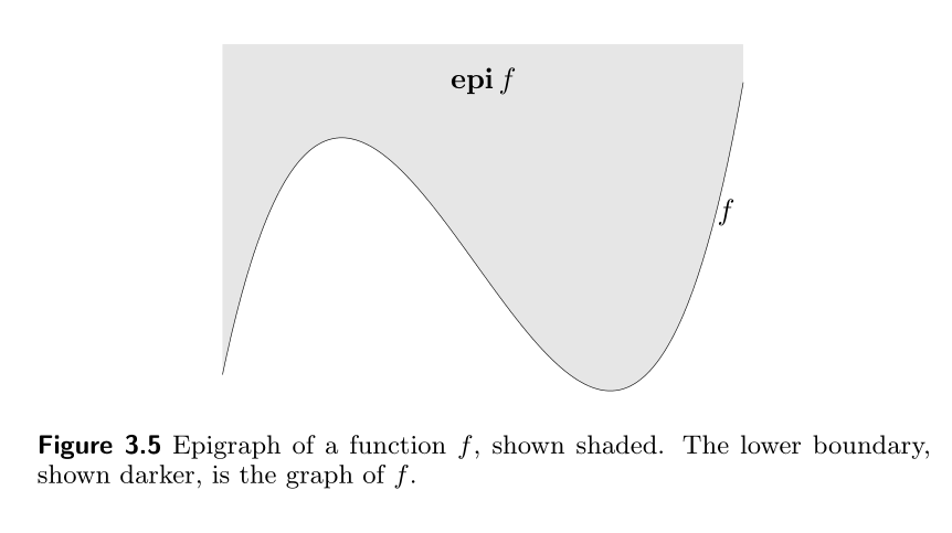
The epigraph of a function $f$: ${\mathbf{R}}^n\to \mathbf{R}$ is defined as e p i   f = { ( x , t ) ∣ x ∈ d o m f , f ( x ) ≤ t } , \mathbf{epi} ~f =\{ (x,t) | x \in \mathbf{dom} f, f(x) \leq t \}, epi f={(x,t)∣x∈domf,f(x)≤t}, which is a subset of ${\mathbf{R}}^{n+1}$, as shown in the following Fig. 3.5.
Note that ‘Epi’ means ‘above’ so epigraph means ‘above the graph’.

The link between convex sets and convex functions is via the epigraph:

• A function is convex if and only its epigraph is convex set.
• A function is concave if and only if its hypograph, defined as, h y p o f = { ( x , t ) ∣ t ≤ f ( x ) } , \mathbf{hypo} f = \{ (x,t) | t \leq f(x) \}, hypof={(x,t)∣t≤f(x)}, is a convex set.

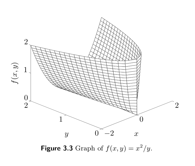
Eaxmple 3.4. Matrix fractional function. The function $f$: ${\mathbf{R}}^n\times {\mathbf{S}}^n\to \mathbf{R}$, defined as, $$f(x,Y)=x^T{Y}^{-1}x$$ is convex on $\mathbf{d}\mathbf{o}\mathbf{m}f={\mathbf{R}}^n\times {\mathbf{S}}_{++}^n$.

One easy way to establish convexity of $f$ is via its epigraph: $$\begin{array}{ll}\mathbf{e}\mathbf{p}\mathbf{i}& =\left\{(x,Y,t)|Y\succ 0,x^T{Y}^{-1}x\le t\right\}\\ & =\left\{(x,Y,t)|\left[\begin{array}{c}Yx\\ x^{T}t\end{array}\right]⪰0,Y\succ 0\right\}\end{array}$$ using the Schur complement condition for positive semidefiniteness of a block matrix.

The last condition is a linear matrix inequality in $(x,Y,t)$, and therefore $\mathbf{e}\mathbf{p}\mathbf{i}f$ is convex.

For the special case $n=1$, the matrix fractional function reduces to the quadratic-over-linear function $x^2/y$, and the associated LMI representation is $$\left[\begin{array}{l}yx\\ xt\end{array}\right]⪰0,y>0$$ (the graph of which is shown in the following figure $3.3$).

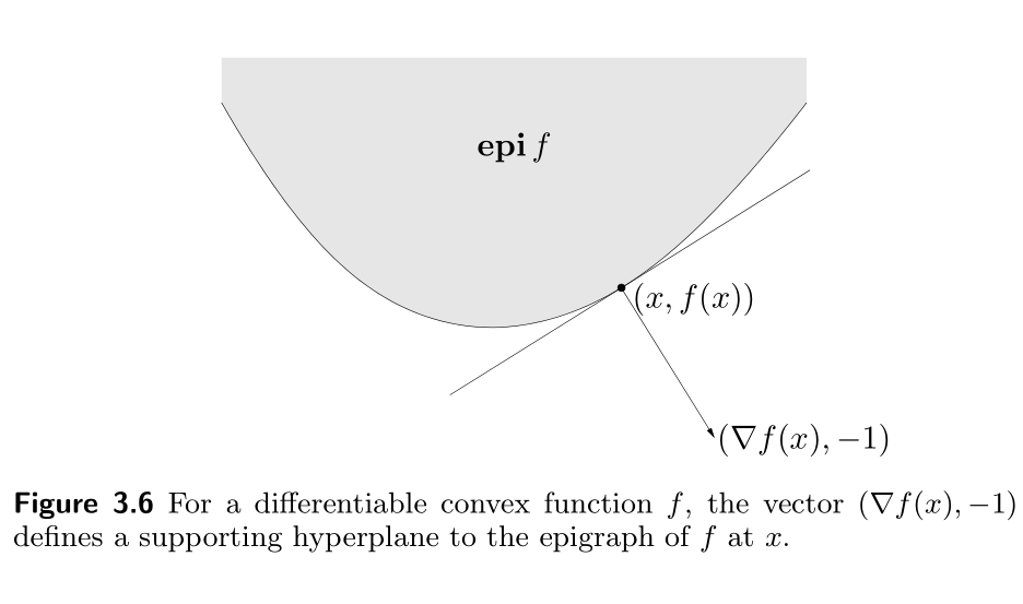
Many results for convex functions can be proved (or interpreted) geometrically using epigraphs, and applying results for convex sets.

As an example, consider first-order condition for the convexity:
$$f(y)\ge f(x)+\nabla f(x)(y-x),$$ where $f$ is convex and $x,y\in \mathbf{d}\mathbf{o}\mathbf{m}f$.

We can interpret this basic inequality geometrically in terms of $\mathbf{e}\mathbf{p}\mathbf{i}f$.
If $(y.t)\in \mathbf{e}\mathbf{p}\mathbf{i}f,$ then $$t\ge f(y)\ge f(x)+\nabla f(x)(y-x).$$
We can express this as:
$$(y,t)\in \mathbf{e}\mathbf{p}\mathbf{i}f\to {\left[\begin{array}{c}\nabla f(x)\\ -1\end{array}\right]}^T\left(\left[\begin{array}{l}y\\ t\end{array}\right]-\left[\begin{array}{c}x\\ f(x)\end{array}\right]\right)\le 0$$
This means that the hyperplane defined by $(\nabla f(x),-1)$ supports epif at the boundary point $(x,f(x))$; see figure 3.6.

---

3.1.8 Jensen’s Inequality and Extensions（延森不等式）

The basic inequality $(3.1)$, i.e., $$f(\theta x+(1-\theta )y)\le \theta f(x)+(1-\theta )f(y),$$ is sometimes called Jensen’s inequality.

It’s easily extended to convex combinations of more than two points: If $f$ is convex, $x_1,...,x_k\in \mathbf{d}\mathbf{o}\mathbf{m}f,$ and ${\theta }_1,...,{\theta }_k\ge 0$ with ${\theta }_1,...,{\theta }_k=1,$ then $$f({\theta }_1{x}_1+....+{\theta }_k{x}_k)\le {\theta }_{1}f(x_1)+...+{\theta }_{k}f(x_k).$$

As in the case of convex sets, the inequality extends to infinite sums, integrals, and expected values. For example, if $p(x)\ge 0$ on $S\subseteq \mathbf{d}\mathbf{o}\mathbf{m}f$, ${\int }_{S}p(x)\text{d}x=1$, then $$f\left({\int }_{S}p(x)x\text{d}x\right)\le {\int }_{S}p(x)f(x)\text{d}x$$ provided the integrals exist.

In the most general case, we can take any probability measure with support in $\mathbf{d}\mathbf{o}\mathbf{m}f$. If $x$ is a random variable such that $x\in \mathbf{d}\mathbf{o}\mathbf{m}f$ with probability one, and $f$ is convex, then we have f ( E { x } ) ≤ E { f ( x ) } f(\mathbb{E}\{x\})\leq \mathbb{E}\{ f(x) \} f(E{x})≤E{f(x)} provided the expectations exist.

Thus, the inequality $(3.5)$ characterizes the convexity: If $f$ is not convex, there is a random variable $x$, with $x\in \mathbf{d}\mathbf{o}\mathbf{m}f$ with probability one, such that f ( E { x } ) > E ( f ( x ) ) . f(\mathbb{E} \{x\}) > \mathbb{E}(f(x)). f(E{x})>E(f(x)).

All of these inequalities are now called Jensen’s inequality, even though the inequality studied by Jensen was the very simple one $$f\left(\frac{x+y}{2}\right)\le \frac{1}{2}f(x)+\frac{1}{2}f(y).$$

Jensen不等式的一般形式：如果$f$是凸函数，$x$是随机变量，那么$f\left(E(x)\right)\le E(f(x))$。

另一种描述：假设$n$个样本 { x 1 , x 2 , . . . , x n } \{x_1,x_2,...,x_n\} {x1​,x2​,...,xn​}和对应的权重 { α 1 , α 2 , . . . , α n } \{\alpha_1,\alpha_2,...,\alpha_n\} {α1​,α2​,...,αn​}，权重满足$\sum {\alpha }_i=1$，对于凸函数$f$，以下不等式成立：
$$f(\sum _{i=1}^n{\alpha }_i{x}_i)\le \sum _{i=1}^n{\alpha }_{i}f(x_i).$$

---

3.1.9 Inequalities

Many famous inequalities can be derived by applying Jensen’s inequality to some appropriate convex functions.

Indeed, convexity and Jensen’s inequality can be made the foundation of a theory of inequalities.

As a simple example, consider the arithmetic-geometric mean inequality: $\sqrt{ab}=a^{\frac{1}{2}}{b}^{\frac{1}{2}}\le \frac{1}{2}a+\frac{1}{2}b$ for $a,b>0$.

The function $-\log x$ is convex; Jensen’s inequality with $\theta =1/2$ yields $-\log (\frac{a+b}{2})\le -\frac{\log a+\log b}{2}$

---

3.2 Operations that preserve convexity（保凸操作）

3.2.1 Nonnegative weighted sums（非负的加权和）

• Evidently, if $f$ is a convex function and $\alpha >0$, then the function $\alpha f$ is convex.
• If $f_1$ and $f_2$ are both convex functions, then so is their sum $f_1+f_2$.
• Combining nonnegative scaling and addition, we see that the set of convex functions is itself a convex cone: a nonnegative weighted sum of convex functions, i.e., $$f=w_1{f}_1+...+w_m{f}_m$$ is convex.
• Similarly, a nonnegative weighted sum of concave functions is concave.
• A nonnegative, nonzero weighted sum of strictly convex (concave) functions is strictly convex (concave).

These properties extend to infinite sums and integrals. For example if $f(x,y)$ is convex in $x$ for each $y\in A$, and $w(y)\ge 0$ for each $y\in A$, then the function $g$ defined as $$g(x)={\int }_{\mathcal{A}}w(y)f(x,y)\text{d}y$$ is convex in $x$ (provided the integral exists).

The fact that convexity is preserved under nonnegative scaling and addition is easily verified directly, or can be seen in terms of the associated epigraphs. For example, if $w\ge 0$ and $f$ is convex, we have
$$\mathrm{epi}(wf)=\left[\begin{array}{cc}I& 0\\ 0& w\end{array}\right]\mathbf{e}\mathbf{p}\mathbf{i}(f)$$ which is convex because the image of a convex set under a linear mapping is convex.

---

3.2.2 Composition with an affine mapping （仿射映射的组合）

Suppose $f$: ${\mathbf{R}}^n\to \mathbf{R}$, $A\in {\mathbf{R}}^{n\times m}$, and $b\in {\mathbf{R}}^n$. Define $g$: ${\mathbf{R}}^m\to \mathbf{R}$ by $$g(x)=f(Ax+b),$$ with d o m g = { x ∣ A x + b ∈ d o m f } . \mathbf{dom} g=\{ x | Ax + b \in \mathbf{dom } f\}. domg={x∣Ax+b∈domf}. Then, if $f$ is convex/concave, so is $g$.

---

3.2.3 Pointwise Maximum and Supremum （点态最大值与上界）

If $f_1$ and $f_2$ are convex functions, then their pointwise maximum $f$, defined by
f ( x ) + max ⁡ { f 1 ( x ) , f 2 ( x ) } , f(x) + \max \{ f_1(x), f_2(x)\}, f(x)+max{f1​(x),f2​(x)}, with $\mathbf{d}\mathbf{o}\mathbf{m}{f}_1\cap \mathbf{d}\mathbf{o}\mathbf{m}{f}_2$, is also convex. This property is easily verified: if $0\le \theta \le 1$ and $x$, $y\in \mathbf{d}\mathbf{o}\mathbf{m}f$, then f ( θ x + ( 1 − θ ) y ) = max ⁡ { f 1 ( θ x + ( 1 − θ ) y ) , f 2 ( θ x + ( 1 − θ ) y ) } ≤ max ⁡ { θ f 1 ( x ) + ( 1 − θ ) f 1 ( y ) , θ f 2 ( x ) + ( 1 − θ ) f 2 ( y ) } ≤ θ max ⁡ { f 1 ( x ) , f 2 ( x ) } + ( 1 − θ ) max ⁡ { f 1 ( y ) , f 2 ( y ) } = θ f ( x ) + ( 1 − θ ) f ( y ) , \begin{aligned} f(\theta x+(1-\theta) y) &=\max \left\{f_{1}(\theta x+(1-\theta) y), f_{2}(\theta x+(1-\theta) y)\right\} \\ & \leq \max \left\{\theta f_{1}(x)+(1-\theta) f_{1}(y), \theta f_{2}(x)+(1-\theta) f_{2}(y)\right\} \\ & \leq \theta \max \left\{f_{1}(x), f_{2}(x)\right\}+(1-\theta) \max \left\{f_{1}(y), f_{2}(y)\right\} \\ &=\theta f(x)+(1-\theta) f(y), \end{aligned} f(θx+(1−θ)y)​=max{f1​(θx+(1−θ)y),f2​(θx+(1−θ)y)}≤max{θf1​(x)+(1−θ)f1​(y),θf2​(x)+(1−θ)f2​(y)}≤θmax{f1​(x),f2​(x)}+(1−θ)max{f1​(y),f2​(y)}=θf(x)+(1−θ)f(y),​ which establishes convexity of $f$. It is easily shown that if $f_1,f_2,...,f_m$ are convex, then their pointwise maximum f ( x ) = max ⁡ { f 1 ( x ) , . . . . , f m ( x ) } f(x) = \max \{ f_1(x), ....,f_m(x) \} f(x)=max{f1​(x),....,fm​(x)} is also convex.

---

---