pytorch搭建深度学习网络

最新推荐文章于 2024-05-30 19:01:13 发布

Nicholson07

最新推荐文章于 2024-05-30 19:01:13 发布

阅读量1.9k

点赞数 1

分类专栏：环境搭建深度学习文章标签： python 深度学习

本文链接：https://blog.csdn.net/Nichlson/article/details/119414042

版权

环境搭建同时被 2 个专栏收录

11 篇文章 2 订阅

订阅专栏

深度学习

8 篇文章 11 订阅

订阅专栏

1、tensor

2、损失函数

1）nn.CrossEntropyLoss

一、Pytorch基础

根据博主的《深度学习入门-基于Python的理论与实现》读书笔记可知，深度学习网络需要经过多次前向传播和反向传播的过程，其中前向传播需要使用损失函数判断训练效果、收敛性，反向传播是一个梯度更新过程（也就是求导过程）。pytorch中封装了多个模块，实现以上功能，另外，还提供了优化器、网络模型库等模块。

1、tensor

张量，是Pytorch中的基本操作对象，可以看作是包含单一数据类型元素的多维矩阵，与numpy的ndarrays很相似，互相之间可以自由转换，但是tensor还支持GPU加速。

#注意，a、b共享地址，修改其中一个，另一个也会改变

import torch
a = torch.ones(5)
b = a.numpy()

import numpy as np
a = np.ones(5)
b = torch.from_numpy(a)

创建张量，可以使用下标索引

a = torch.Tensor(2,2)#基础tensor

b = torch.DoubleTensor(2,2)#指定类型

c = torch.Tensor([[1,2],[3,4]]) #使用list创建

d = torch.zeros(2,2) #默认值为0

e = torch.ones(2,2) #默认值为1

f = torch.eye(2,2) #对角张量

g = torch.randn(2,2) #随机张量

h = torch.randperm(n) #随机排列张量，0-n整数，随机排列的一维张量

2、损失函数

pytorch在torch.nn及torch.nn.functional中包含了各种损失函数，通常来讲，损失函数不含有可学习的参数。

对于同一种损失函数，使用nn.xx或nn.functional.xx来实现，其功能是一样的。两者的关系在于torch.nn.functional中直接写了函数的实现，而torch.nn中是用类封装了torch.nn.functional中的函数。因此torch.nn需要先实例化，再调用函数，而torch.nn.functional可以直接调用函数。一般来讲，直接使用torch.nn就够了，个人觉得尽量使用torch.nn，但是由于torch.nn多了一层类的封装，灵活性不如torch.nn.functional，所以有时也需要使用到。

常用损失函数：

1）nn.CrossEntropyLoss

交叉熵：它主要刻画的是实际输出（概率）与期望输出（概率）的距离，也就是交叉熵的值越小，两个概率分布就越接近。假设概率分布p为期望输出，概率分布q为实际输出， $H(p,q)$ 为交叉熵，则

$H(p,q)=\sum_{x}^{}p(x)logq(x)$

#CrossEntropyLoss()
criterion = nn.CrossEntropyLoss()
input = torch.Tensor([[-0.7715, -0.6205, -0.2562]])
target = torch.tensor([0])
output = criterion (input, target)

2）nn.L1Loss

$loss(xi,yi)=\left | xi-yi \right |$

#L1Loss
loss = nn.L1Loss(reduction='sum')
input = torch.tensor([1., 2, 3, 4])
target = torch.tensor([4., 5, 6, 7])
output = loss(input, target)

3）nn.MSELoss

$loss(xi,yi)=(xi-yi)^{2}$

#MSELoss
a = torch.tensor([1., 2, 3, 4])
b = torch.tensor([4., 5, 6, 7])
loss_fn = nn.MSELoss(reduce=True, size_average=True)
loss = loss_fn(a, b)

3、自动求导Autograd

基于链式法则，自动求取反向传播过程中需要的导数。这里需要知道tensor的一个属性requires_grad，默认为False。

参数requires_grad 的含义及标志位说明：

1.如果对于某        变量 x ，其 x.requires_grad == True , 则表示它可以参与求导，也可以从它向后求导。默认情况下，一个新的Variables 的 requires_grad 和 volatile 都等于 False 。
2.requires_grad == True 具有传递性，例如：
        x.requires_grad == True ，y.requires_grad == False ， z=f(x,y)
        则， z.requires_grad == True。
3.凡是参与运算的变量（包括输入量，中间输出量，输出量，网络权重参数等），都可以设置 requires_grad 。
4.volatile==True 就等价于 requires_grad==False 。 volatile==True 同样具有传递性。一般只用在inference（推理）过程中。若是某个过程，从 x 开始都只需做预测，不需反传梯度的话，那么只需设置x.volatile=True ，那么 x 以后的运算过程的输出均为 volatile==True ,即 requires_grad==False 。
        由于inference 过程不必backward()，所以requires_grad 的值为False 或 True，对结果是没有影响的，但是对程序的运算效率有直接影响；因此，在inference过程中，使用volatile=True ，就不必把运算过程中所有参数都手动设一遍requires_grad=False 了，方便快捷。
5.detach() ：如果 x 为中间输出，x’ = x.detach 表示创建一个与 x 相同，但requires_grad==False 的variable，(实际上是把x’ 以前的计算图 grad_fn 都消除了)，x’ 也就成了叶节点。原先反向传播时，回传到x时还会继续，而现在回到x’处后，就结束了，不继续回传求到了。另外值得注意，x (variable类型) 和 x’ (variable类型)都指向同一个Tensor ,即 x.data，因此，detach_() 表示不创建新变量，而是直接修改 x 本身。
6.retain_graph：每次 backward() 时，默认会把整个计算图free掉。一般情况下是每次迭代，只需一次 forward() 和一次 backward() ，前向运算forward() 和反向传播backward()是成对存在的，一般一次backward()也是够用的。但是不排除，由于自定义loss等的复杂性，需要一次forward()之后，通过多个不同loss的backward()来累积同一个网络的grad，进行参数更新。于是，若在当前backward()后，不执行forward() 而可以执行另一个backward()，需要在当前backward()时，指定保留计算图，即backward(retain_graph)。

参考链接:PyTorch中关于backward、grad、autograd的计算原理的深度剖析_Yale-曼陀罗-CSDN博客

调用.backward()时会从模型的output开始反向计算，直到前一个变量的requires_grad=False时停止。

注意，模型输出Output的requires_grad=True，而用户定义的输入值通常为False。

官网示例如下：

import torch


# N is batch size; D_in is input dimension;
# H is hidden dimension; D_out is output dimension.
N, D_in, H, D_out = 64, 1000, 100, 10

# Create random Tensors to hold inputs and outputs
x = torch.randn(N, D_in)
y = torch.randn(N, D_out)

# Use the nn package to define our model as a sequence of layers. nn.Sequential
# is a Module which contains other Modules, and applies them in sequence to
# produce its output. Each Linear Module computes output from input using a
# linear function, and holds internal Tensors for its weight and bias.

# 最简单的只有1层隐藏层的序惯模型

model = torch.nn.Sequential(
    torch.nn.Linear(D_in, H),
    torch.nn.ReLU(),
    # 最后一层后面也要加逗号——————,
    torch.nn.Linear(H, D_out),
)

# loss_function定义 size_average的说明见上面，也就是只算每个batch size的总loss。
loss_fn = torch.nn.MSELoss(size_average=False)
learning_rate = 1e-4

# 相当于将batchsize为64的数据喂入模型500次，即epoch=500
# 这里的权值更新很直观，torch.no_grad()每个参数直接执行 param -= learning_rate * param.grad
for t in range(500):
    # Forward pass: compute predicted y by passing x to the model. Module objects
    # override the __call__ operator so you can call them like functions. When
    # doing so you pass a Tensor of input data to the Module and it produces
    # a Tensor of output data.

    # 0.4.0版本已经将 Variable 和 Tensor合并，统称为 Tensor
    y_pred = model(x)

    # Compute and print loss. We pass Tensors containing the predicted and true
    # values of y, and the loss function returns a Tensor containing the
    # loss.
    loss = loss_fn(y_pred, y)
    print('round', t+1, loss.item())

    # Zero the gradients before running the backward pass.
    model.zero_grad()

    # Backward pass: compute gradient of the loss with respect to all the learnable
    # parameters of the model. Internally, the parameters of each Module are stored
    # in Tensors with requires_grad=True, so this call will compute gradients for
    # all learnable parameters in the model.
    loss.backward()

    # 手动调整模型参数 当然，我们可以用optim包去定义Optimizer并自动帮助我们更新权值。optim包里包括了SGD+momentum, RMSProp, Adam等常见的深度学习优化算法.
    with torch.no_grad():
        for param in model.parameters():
            param -= learning_rate * param.grad

nn.optim中包含了各种常见的优化算法，包括常用算法包括随机梯度下降算法SGC（Stochastic Gradient Descent）、Adam（Adaptive Moment Estimation）等。

SGD是一种梯度下降法，是指沿着梯度下降的方向求解极小值，一般用于求解最小二乘问题。通常以一个小批次数据为单位，可计算一个批次的梯度，然后反向传播。优点是只需要小批量数据即可实现，计算量小，收敛速度快。缺点是依赖一个较好的初始学习率，但是这个值不直观，不容易选择，另外容易陷入局部最小。为了解决第二个缺点，通常的做法是增加动量，也就是当此次梯度方向与上次相同时，梯度会变大，会加快收敛，而反之，梯度会变小，抑制震荡，增加稳定性。由于在训练的中后期，梯度会在局部极小值周围震荡，此时梯度接近0，但动量的存在使得梯度更新不是0，才有可能跳出局部最小。

Adam利用梯度的一阶矩与二阶矩动态地调整每一个参数的学习率，是一种学习率自适应算法，优点在于，经过调整后，每一次迭代的学习率都在一个确定范围内，使得参数更新更加平稳。此外，还可以使模型更快受凉，尤其适用于一些深层网络。

下面的代码采用optim包的优化器更新权值的实例。

import torch

# N is batch size; D_in is input dimension;
# H is hidden dimension; D_out is output dimension.
N, D_in, H, D_out = 64, 1000, 100, 10

# Create random Tensors to hold inputs and outputs
x = torch.randn(N, D_in)
y = torch.randn(N, D_out)

# Use the nn package to define our model and loss function.
model = torch.nn.Sequential(
    torch.nn.Linear(D_in, H),
    torch.nn.ReLU(),
    torch.nn.Linear(H, D_out),
)
loss_fn = torch.nn.MSELoss(size_average=False)

# Use the optim package to define an Optimizer that will update the weights of
# the model for us. Here we will use Adam; the optim package contains many other
# optimization algoriths. The first argument to the Adam constructor tells the
# optimizer which Tensors it should update.
learning_rate = 1e-4

# 优化器，AdamOptimizer
optimizer = torch.optim.Adam(model.parameters(), lr=learning_rate) 

for t in range(500):
    # Forward pass: compute predicted y by passing x to the model.
    y_pred = model(x)

    # Compute and print loss.
    loss = loss_fn(y_pred, y)
    print(t, loss.item())

    # Before the backward pass, use the optimizer object to zero all of the
    # gradients for the variables it will update (which are the learnable
    # weights of the model). This is because by default, gradients are
    # accumulated in buffers( i.e, not overwritten) whenever .backward()
    # is called. Checkout docs of torch.autograd.backward for more details.
    # 原来是model.zero_grad()
    optimizer.zero_grad()

    # Backward pass: compute gradient of the loss with respect to model
    # parameters
    loss.backward()

    # 调用Optimizer的step function来更新Model的权值。
    optimizer.step()

4、网络模型库torchvision

torchvision.models提供了众多经典网络结构与预训练模型，如VGG、ResNet等，利用这些模型可以快速搭建物体检测网络。

1）加载预训练模型

可以从官网加载预训练好的模型：

import torchvision.models as models

#第一种，加载完整模型
model= models.resnet50(pretrained=True) 

#第二种，加载模型结构，但不包含预训练参数
model = models.resnet50(pretrained=False) 

#第三种，加载模型结构和部分预训练参数
resnet50 = models.resnet50(pretrained=True) 
model = Net(...) #Net是自己定义的模型
 
pretrained_dict =resnet50.state_dict() #读取预训练模型参数,字典格式（键值）
model_dict = model.state_dict()  

pretrained_dict =  {k: v for k, v in pretrained_dict.items() if k in model_dict} #将pretrained_dict里不属于model_dict的键剔除掉
 
model_dict.update(pretrained_dict) #更新model_dict
 
model.load_state_dict(model_dict) #加载参数

从上面第三种方式不难发现，我们也可以从本地加载预训练模型：

import torchvision.models as models
 
model = models.vgg16(pretrained=False) #加载网络结构
pre = torch.load(r'.\kaggle_dog_vs_cat\pretrain\vgg16-397923af.pth') #从本地预训练模型读取参数
model.load_state_dict(pre) #将参数赋予自己的模型

通用下载网址vision/torchvision/models at main · pytorch/vision · GitHub

常用模型及地址

Resnet:

model_urls = {
    'resnet18': 'https://download.pytorch.org/models/resnet18-5c106cde.pth',
    'resnet34': 'https://download.pytorch.org/models/resnet34-333f7ec4.pth',
    'resnet50': 'https://download.pytorch.org/models/resnet50-19c8e357.pth',
    'resnet101': 'https://download.pytorch.org/models/resnet101-5d3b4d8f.pth',
    'resnet152': 'https://download.pytorch.org/models/resnet152-b121ed2d.pth',
}
 
inception:

model_urls = {
    # Inception v3 ported from TensorFlow
    'inception_v3_google': 'https://download.pytorch.org/models/inception_v3_google-1a9a5a14.pth',
}

Densenet:

model_urls = {
    'densenet121': 'https://download.pytorch.org/models/densenet121-a639ec97.pth',
    'densenet169': 'https://download.pytorch.org/models/densenet169-b2777c0a.pth',
    'densenet201': 'https://download.pytorch.org/models/densenet201-c1103571.pth',
    'densenet161': 'https://download.pytorch.org/models/densenet161-8d451a50.pth',
}



Alexnet:

model_urls = {
    'alexnet': 'https://download.pytorch.org/models/alexnet-owt-4df8aa71.pth',
}

vggnet:

model_urls = {
    'vgg11': 'https://download.pytorch.org/models/vgg11-bbd30ac9.pth',
    'vgg13': 'https://download.pytorch.org/models/vgg13-c768596a.pth',
    'vgg16': 'https://download.pytorch.org/models/vgg16-397923af.pth',
    'vgg19': 'https://download.pytorch.org/models/vgg19-dcbb9e9d.pth',
    'vgg11_bn': 'https://download.pytorch.org/models/vgg11_bn-6002323d.pth',
    'vgg13_bn': 'https://download.pytorch.org/models/vgg13_bn-abd245e5.pth',
    'vgg16_bn': 'https://download.pytorch.org/models/vgg16_bn-6c64b313.pth',
    'vgg19_bn': 'https://download.pytorch.org/models/vgg19_bn-c79401a0.pth',
}

2）自己模型的保存与加载

有两种方法，第一种只保存和加载模型中的参数

#保存
torch.save(resnet50.state_dict(),'ckp/model.pth')   

#加载
resnet=resnet50(pretrained=True)
resnet.load_state_dict(torch.load('ckp/model.pth'))

第二种同时保存和加载模型的结构和参数

# 保存
torch.save (model, 'ckp/model.pth')

# 加载
model = torch.load('ckp/model.pth')

5、数据处理

常见公开数据集包括ImageNet、PASCAL VOC、COCO等。

1）数据加载

分为三步，继承Dataset类（获取可迭代的数据集），数据变换与增强torchvision.transforms、继承dataloader（实际使用的实例）。

继承Dataset并重写__len__()和__getitem__()函数，可以实现数据集迭代的底层模块。

from torch.utils.data import Dataset
class my_data(Dataset):
    def __init__(self, image_path, annotation_path, transform=None):
        # 初始化，读取数据集
    def __len__(self):
        # 获取数据集的总大小
    def __getitem__(self, id):
        # 对于指定的id，读取并返回该数据

Dataset只是将数据集加载到了实例中，实际使用时，数据集中的图片可能存在大小不一等情况，需要进行一些处理。

from torchvision import transforms
#可以将transforms集合到Dataset中，并使用Compose将多个变换整合在一起
dataset = my_data("your image path", "your annotation path", transforms=
                 transforms.Compose([
                 transforms.Resize(256)#将图像最短边缩小至256，宽高比不变
                 transforms.RandomHorizontalFlip()#以0.5的概率翻转指定的PIL图像
                 transforms.ToTensor()#将PIL图像转换为Tensor，元素区间从[0,255]归一到[0,1]
                 transforms.Normalize([0.5, 0.5, 0.5], [0.5, 0.5, 0.5])#进行mean与std为0.5的标准化
                 ]))

经过前两步可以获取每一个变换后的样本，但是仍然无法进行批处理、随机选取等操作，因此还需要进一步封装。

from torch.utils.data import Dataloader

dataloader = Dataloader(dataset, batch_Size=4, shuffle=True, num_workers=4)

#第一种方式
data_iter = iter(dataloader)
for step in range(iters_per_epoch):
    data = next(data_iter)

#第二种方式
for idx, (img, label) in enumerate(dataloader)
    #这里的（img, label）与dataset中__getitem__函数的返回值对应

2）GPU加速

可以使用torch.cuda.is_available()来判断当前环境下GPU是否可用，对于Tensor和模型，可以直接调用cuda()方法将数据转移到GPU上运行，还可以使用具体数字指定转移到哪一个GPU上。

import torch
from torchvision import models

a = torch.randn(3,3)
b = models.vgg16()

if torch.cuda.is_available():

    a = a.cuda()
    b = b.cuda(1)#第一种方式指定到GPU1

    #第二种方式，指定到GPU1
    device = torch.device("cuda:1")
    c = torch.randn(3, 3 device = device)

6、导出onnx

1）导出onnx

Open Neural Network Exchange（ONNX，开放神经网络交换）格式，是一个用于表示深度学习模型的标准，可使模型在不同框架之间进行转移。

ONNX是一种针对机器学习所设计的开放式的文件格式，用于存储训练好的模型。它使得不同的人工智能框架（如Pytorch, MXNet）可以采用相同格式存储模型数据并交互。 ONNX的规范及代码主要由微软，亚马逊，Facebook 和 IBM 等公司共同开发，以开放源代码的方式托管在Github上。目前官方支持加载ONNX模型并进行推理的深度学习框架有： Caffe2, PyTorch, MXNet，ML.NET，TensorRT 和 Microsoft CNTK，并且 TensorFlow 也非官方的支持ONNX。---维基百科

因此，为了完成模型的部署，有时需要将pth文件转换成onnx。

import torch

model_path = r"L:\testmodel\model\model.pth" # 待转换的模型
onnx_path = r"L:\testmodel\model\model.onnx" # 存放onnx模型的位置

model = torch.load(model_path)
model.eval()

device = torch.device("cuda:0" if torch.cuda.is_available() else "cpu")
input = torch.ones(1,3,224,224).to(device)

torch.onnx.export(model, input. onnx_path,
                  opset_version=10,
                  verbose=True,                                # 打印网络结构
                  input_names=["input"],
                  output_names=["output"],
                  dynamic_axes={"input": {0: "batch_size"},    # 动态维度
                                "output": {0: "batch_size"}})

运行成功后就类似如下

D:\Anaconda3\envs\pytorch\python.exe L:/testmodel/pth_2_onnx.py
graph(%input_1 : Float(1, 3, 224, 224),
      %conv1.weight : Float(16, 3, 5, 5),
      %conv1.bias : Float(16),
      %conv2.weight : Float(32, 16, 5, 5),
      %conv2.bias : Float(32),
      %fc1.weight : Float(120, 89888),
      %fc1.bias : Float(120),
      %fc2.weight : Float(84, 120),
      %fc2.bias : Float(84),
      %fc3.weight : Float(2, 84),
      %fc3.bias : Float(2)):
  %11 : Float(1, 16, 220, 220) = onnx::Conv[dilations=[1, 1], group=1, kernel_shape=[5, 5], pads=[0, 0, 0, 0], strides=[1, 1]](%input_1, %conv1.weight, %conv1.bias), scope: LeNet/Conv2d[conv1]
  %12 : Float(1, 16, 220, 220) = onnx::Relu(%11), scope: LeNet
  %13 : Float(1, 16, 110, 110) = onnx::MaxPool[kernel_shape=[2, 2], pads=[0, 0, 0, 0], strides=[2, 2]](%12), scope: LeNet/MaxPool2d[pool1]
  %14 : Float(1, 32, 106, 106) = onnx::Conv[dilations=[1, 1], group=1, kernel_shape=[5, 5], pads=[0, 0, 0, 0], strides=[1, 1]](%13, %conv2.weight, %conv2.bias), scope: LeNet/Conv2d[conv2]
  %15 : Float(1, 32, 106, 106) = onnx::Relu(%14), scope: LeNet
  %16 : Float(1, 32, 53, 53) = onnx::MaxPool[kernel_shape=[2, 2], pads=[0, 0, 0, 0], strides=[2, 2]](%15), scope: LeNet/MaxPool2d[pool2]
  %17 : Float(1, 89888) = onnx::Flatten[axis=1](%16), scope: LeNet
  %18 : Float(1, 120) = onnx::Gemm[alpha=1, beta=1, transB=1](%17, %fc1.weight, %fc1.bias), scope: LeNet/Linear[fc1]
  %19 : Float(1, 120) = onnx::Relu(%18), scope: LeNet
  %20 : Float(1, 84) = onnx::Gemm[alpha=1, beta=1, transB=1](%19, %fc2.weight, %fc2.bias), scope: LeNet/Linear[fc2]
  %21 : Float(1, 84) = onnx::Relu(%20), scope: LeNet
  %output_1 : Float(1, 2) = onnx::Gemm[alpha=1, beta=1, transB=1](%21, %fc3.weight, %fc3.bias), scope: LeNet/Linear[fc3]
  return (%output_1)


Process finished with exit code 0

遇到的问题：

cannot insert a tensor that requires grad as a constant

解决方式：在构建模型的时候，如果需要使用到List添加模型的层，就必须使用nn.ModuleList代替list，否则虽然模型可以正常训练，但是导出onnx时无法解析。

couldn't export python operator SwishImplementation

解决方式：这是efficientnet本身的问题，他有两个swich函数，分别用于training和exporting。对模型的efficientnet部分调用.set_swish(memory_efficient=False)。

2）测试onnx

想要验证onnx模型与原模型是否一致可以使用onnx和onnxruntime库。

import torch
import onnx
import onnxruntime

onnx_path = r"L:\testmodel\model\model.onnx" # 存放onnx模型的位置
model = onnx.load(onnx_path)
onnx.checker.check_model(onnx_model)

output = onnx_model.graph.output     # 打印onnx模型的输入输出维度
print(output)

img_data = torch.ones(1,3,224,224).numpy()
sess = onnxruntime.InferenceSession(onnx_path)
outputs = sess.run(output_list, {"input": img_data})  # 推理并打印输出结果
print(outputs)

二、网络骨架解析

1、深度学习网络的基本组成

详见《深度学习入门-基于Python的理论与实现》读书笔记第七章。

2、常见网络结构

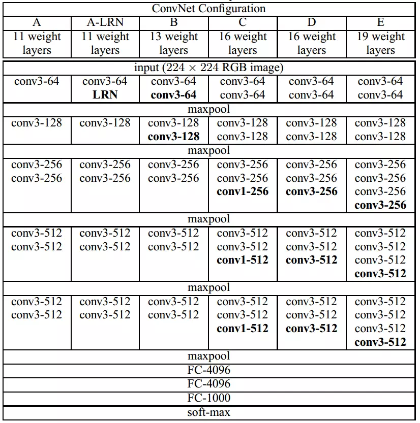
1）VGG

最常用的是VGG16，采用五组卷积与三个全连接层，最后使用Softmax分类。

使用的卷积核基本都是3*3，有些地方出现了多个3*3堆叠的现象，这种结构的优点在于，使用较少的参数实现了与5*5卷积核相同的感受野。

2）Inception

使用多个不同大小的卷积运算，并将不同卷积运算的结果级联起来，送入下一层。以Inception V1为例，一共有9个上述堆叠模块，共有22层。参数量是VGG的1/3，更适合处理大规模数据。

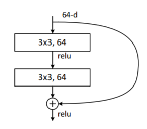
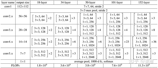
3）ResNet

引入深度残差框架解决网络深度导致的梯度消失问题，即让卷积网络去学习残差映射，而不是期望每一个堆叠层的网络都完整地拟合潜在的映射。

以ResNet50为例，最主要的部分在于中间经历了4个大的卷积组，而这4个卷积组分别包含了3、4、6这三个Bottleneck模块，最后经过一个全局平均池化使得特征图大小变为1*1，然后进行1000维的全连接，最后经过Softmax输出分类得分。

preview

3、经典物体检测框架

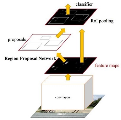
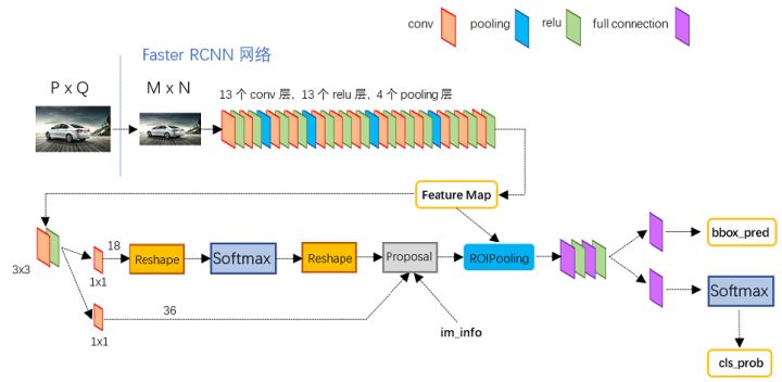
1）两阶经典检测器Faster RCNN

参考这位大佬的文章：一文读懂Faster RCNN

未完待续

参考资料：PyTorch学习笔记(1)——requires_grad和autograd.no_grad

一文读懂Faster RCNN

Nicholson07

关注

1
点赞
踩
16

收藏

觉得还不错? 一键收藏
0
评论
pytorch搭建深度学习网络

预训练模型通用下载网址https://github.com/pytorch/vision/tree/master/torchvision/models 常用模型及地址Resnet:model_urls = { 'resnet18': 'https://download.pytorch.org/models/resnet18-5c106cde.pth', 'resnet34': 'https://download.pytorch.org/mode...
复制链接

扫一扫