python模拟离散傅里叶变换

code：

import numpy as np
import matplotlib as mpl
import matplotlib.pyplot as plt

# 产生三角波的函数
def triangle(size, T):
	# 生成-1到1之间的size个时间点
	t = np.linspace(-1, 1, size, endpoint=False)
	# 这里使用y=|x|函数生成倒三角波一样的图像
	y = np.abs(t)
	# 上面已经生成一个三角波图像,然后进行复制T个
	y = np.tile(y, T) - 0.5
	# 接着吧上面总共采样的T个周期的所有采样点集合到x变量
	x = np.linspace(0, 2 * np.pi * T, size * T, endpoint=False)
	return x, y

# 把采样点的0点去掉
def delete_zero(f):
	f1 = np.real(f)
	f2 = np.imag(f)
	# 设置一个极小接近0的值
	e_min = 1e-5
	# 同上面的极小值比较去0
	return f1[(f1 > e_min) | (f1 < -e_min)], f2[(f2 > e_min) | (f2 < -e_min)]

if __name__ == "__main__":

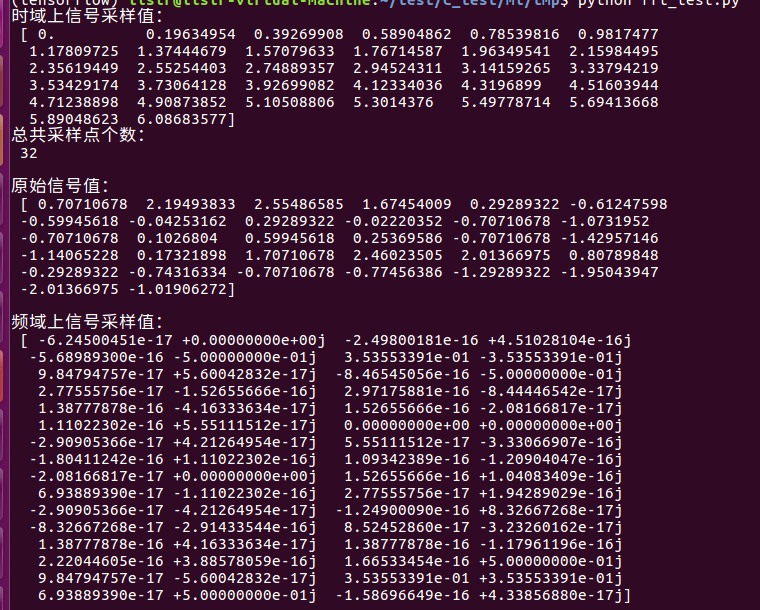
    x = np.linspace(0, 2*np.pi, 32, endpoint=False)
    print('时域上信号采样值：\n', x)
    # y = np.sin(2*x) + np.sin(3*x + np.pi/4) + np.sin(5*x)
    y = np.sin(x)

    N = len(x)
    print('总共采样点个数：\n', N)
    print('\n原始信号值：\n', y)
    f = np.fft.fft(y)
    print('\n频域上信号采样值：\n', f/N)
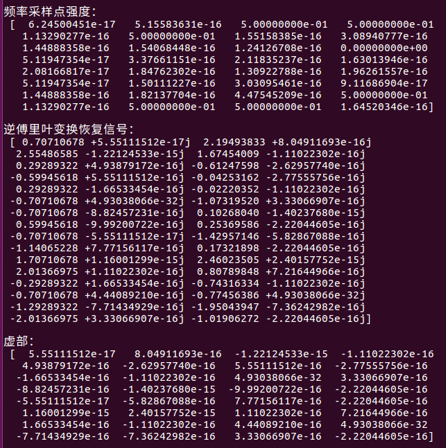
    a = np.abs(f/N)
    print('\n频率采样点强度：\n', a)

    iy = np.fft.ifft(f)
    print('\n逆傅里叶变换恢复信号：\n', iy)
    print('\n虚部：\n', np.imag(iy))
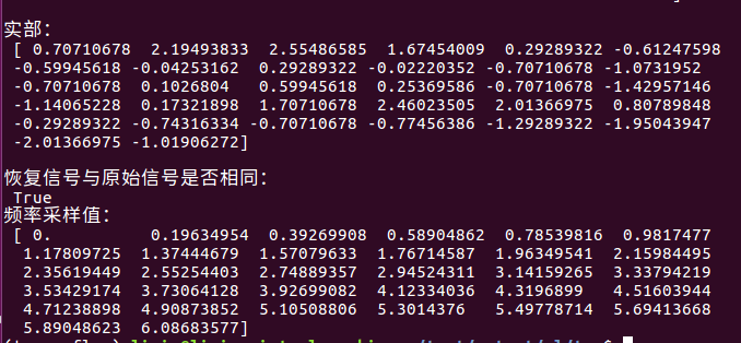
    print('\n实部：\n', np.real(iy))
    print('\n恢复信号与原始信号是否相同：\n', np.allclose(np.real(iy), y))

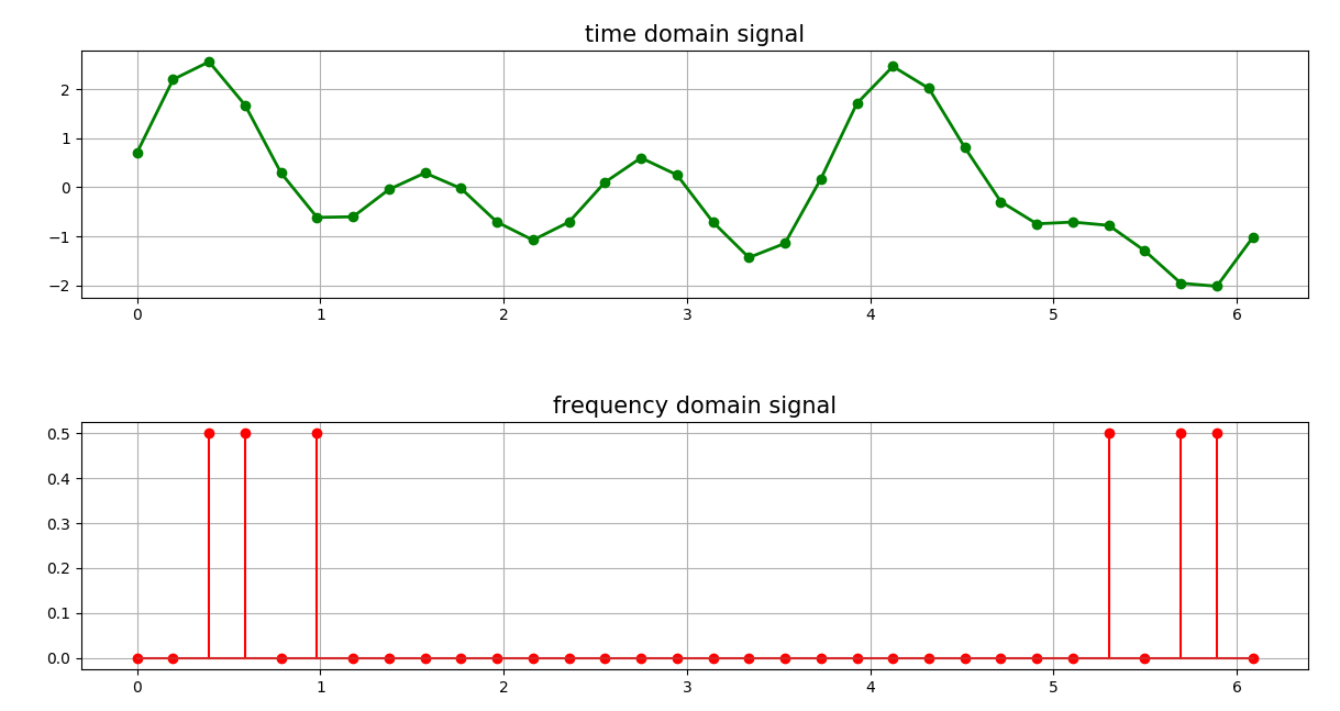
    plt.subplot(211)
    plt.plot(x, y, 'go-', lw=2)
    plt.title('time domain signal', fontsize=15)
    plt.grid(True)
    plt.subplot(212)
    w = np.arange(N) * 2*np.pi / N
    print('频率采样值：\n', w)
    plt.stem(w, a, linefmt='r-', markerfmt='ro')
    plt.title('frequency domain signal', fontsize=15)
    plt.tight_layout(2)  
    plt.subplots_adjust(top=0.9)
    plt.grid(True)
    plt.show()

    # 模拟三角锯齿波
    x, y = triangle(30, 7)
    N = len(y)
    f = np.fft.fft(y)
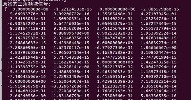
    print("原始的三角频域信号:\n", np.real(f), np.imag(f))
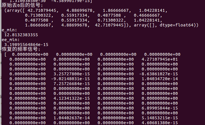
    print("原始去0后的信号:\n", delete_zero(f))
    a = np.abs(f/N)
    
    f_real = np.real(f)
    e_min = 0.3 * f_real.max()
    print("e_min:\n", e_min)
    # 去0处理
    f_real[(f_real < e_min) & (f_real > -e_min)] = 0
    
    f_imag = np.imag(f)
    ee_min = 0.3 * f_imag.max()
    f_imag[(f_imag < ee_min) & (f_imag > -ee_min)] = 0

    print("ee_min:\n", ee_min)
    new_f = f_real + f_imag
    new_y = np.fft.ifft(new_f)
    new_y = np.real(new_y)

    print("恢复的频率信号:\n", new_f)
    print("恢复的去0后的频率信号:\n", delete_zero(new_f))

    plt.figure(figsize=(8, 8), facecolor='w')
    plt.subplot(311)
    plt.plot(x, y, 'g-', linewidth=2)
    plt.title('triangle signal', fontsize=15)
    plt.grid(True)
    plt.subplot(312)
    w = np.arange(N) * 2*np.pi / N
    plt.stem(w, a, lineformat='r-', markerformat='ro')
    plt.title('frequency domain signal', fontsize=15)
    plt.grid(True)
    plt.subplot(313)
    plt.plot(x, new_y, 'b-', lw=2, markersize=4)
    plt.title('triangle restore signal', fontsize=15)
    plt.grid(True)
    plt.tight_layout(1.5, rect=[0, 0.04, 1, 0.96])
    plt.suptitle('quickly fft translation and frequency fliter signal', fontsize=17)
    plt.show()

　　傅里叶变换是信号处理领域的一种极其重要的手段，很多的滤波算法也是基于傅里叶变换而来，通过这个实验我们可以简单模拟傅里叶变换极其逆变换，同时也可以看出低通和高通滤波无非也是讲个别信号抑制，通过设置阈值在滤波中滤掉。