


目录
一、二、Tesnsflow入门 & 环境配置 & 认识Tensorflow
Tensorflow入门(1)——深度学习框架Tesnsflow入门 & 环境配置 & 认识Tensorflow
三、线程与队列与IO操作
深度学习框架Tesnsflow & 线程+队列+IO操作 & 文件读取案例

神经网络基础知识
神经网络的种类:
基础神经网络:单层感知器,线性神经网络,BP神经网络,Hopfield神经网络等
进阶神经网络:玻尔兹曼机,受限玻尔兹曼机,递归神经网络等
深度神经网络:深度置信网络,卷积神经网络,循环神经网络,LSTM网络等
• 结构(Architecture)例如,神经网络中的变量可以是神经元连接的权重
• 激励函数(Activity Rule)大部分神经网络模型具有一个短时间尺度的动力学规则,来定义神经元如何根据其他神经元的活动来改变自己的激励值。
• 学习规则(Learning Rule)学习规则指定了网络中的权重如何随着时间推进而调整。(反向传播算法)

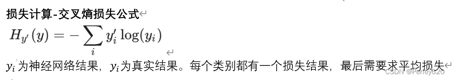
损失计算-交叉熵损失公式
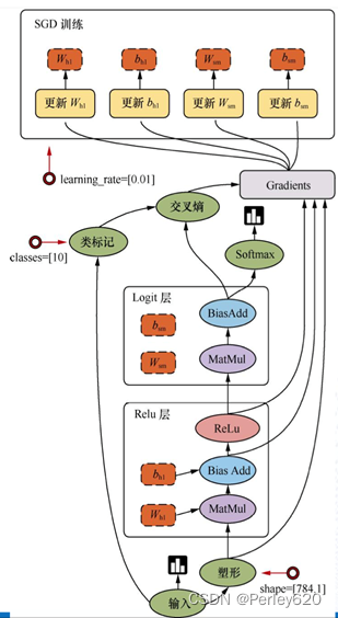
1.简单神经网络
TensorFlow的代码
import tensorflow as tf
old_v = tf.logging.get_verbosity()
tf.logging.set_verbosity(tf.logging.ERROR)
from tensorflow.examples.tutorials.mnist import input_data
FLAGS = tf.app.flags.FLAGS
tf.app.flags.DEFINE_integer("is_train", 1, "指定程序是预测还是训练")
def full_connected():
# 获取真实的数据
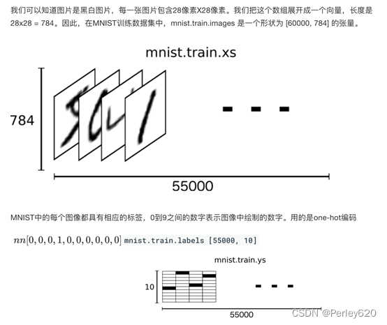
mnist = input_data.read_data_sets("./data/mnist/", one_hot=True)
tf.logging.set_verbosity(old_v)
# 1、建立数据的占位符 x [None, 784] y_true [None, 10]
with tf.variable_scope("data"): # 作用域
x = tf.placeholder(tf.float32, [None, 784])
y_true = tf.placeholder(tf.int32, [None, 10])
# 2、建立一个全连接层的神经网络 w [784, 10] b [10]
with tf.variable_scope("fc_model"):
# 随机初始化权重和偏置
weight = tf.Variable(tf.random_normal([784, 10], mean=0.0, stddev=1.0), name="w")
bias = tf.Variable(tf.constant(0.0, shape=[10]))
# 预测None个样本的输出结果matrix [None, 784]* [784, 10] + [10] = [None, 10]
y_predict = tf.matmul(x, weight) + bias
# 3、求出所有样本的损失,然后求平均值
with tf.variable_scope("soft_cross"):
# 求平均交叉熵损失
loss = tf.reduce_mean(tf.nn.softmax_cross_entropy_with_logits(labels=y_true, logits=y_predict))
# 4、梯度下降求出损失
with tf.variable_scope("optimizer"):
train_op = tf.train.GradientDescentOptimizer(0.1).minimize(loss)# 学习率和最小化损失
# 5、计算准确率
with tf.variable_scope("acc"):
equal_list = tf.equal(tf.argmax(y_true, 1), tf.argmax(y_predict, 1))
# equal_list None个样本 [1, 0, 1, 0, 1, 1,..........]
accuracy = tf.reduce_mean(tf.cast(equal_list, tf.float32))
# 收集变量 单个数字值收集
tf.summary.scalar("losses", loss)
tf.summary.scalar("acc", accuracy)
# 高纬度变量收集
tf.summary.histogram("weightes", weight)
tf.summary.histogram("biases", bias)
# 定义一个初始化变量的op
init_op = tf.global_variables_initializer()
# 定义一个合并变量的 op
merged = tf.summary.merge_all()
# 创建一个saver
saver = tf.train.Saver()
# 开启会话去训练
with tf.Session() as sess:
# 初始化变量
sess.run(init_op)
# 建立events文件,然后写入
filewriter = tf.summary.FileWriter("./tmp/summary/test/", graph=sess.graph)
if FLAGS.is_train == 1:# 如果是1,进行训练
# 迭代步数去训练,更新参数预测
for i in range(2000):
# 取出真实存在的特征值和目标值
mnist_x, mnist_y = mnist.train.next_batch(50)
# 运行train_op训练
sess.run(train_op, feed_dict={x: mnist_x, y_true: mnist_y})
# 写入每步训练的值
summary = sess.run(merged, feed_dict={x: mnist_x, y_true: mnist_y})
filewriter.add_summary(summary, i)
print("训练第%d步,准确率为:%f" % (i, sess.run(accuracy, feed_dict={x: mnist_x, y_true: mnist_y})))
# 保存模型
saver.save(sess, "./tmp/ckpt/fc_model")
else:# 如果是0,做出预测
# 加载模型
saver.restore(sess, "./tmp/ckpt/fc_model")
# 如果是0,做出预测
for i in range(100):
# 每次测试一张图片 [0,0,0,0,0,1,0,0,0,0]
x_test, y_test = mnist.test.next_batch(1)
print("第%d张图片,手写数字图片目标是:%d, 预测结果是:%d" % (
i,
tf.argmax(y_test, 1).eval(),
tf.argmax(sess.run(y_predict, feed_dict={x: x_test, y_true: y_test}), 1).eval()
))
return None
if __name__ == "__main__":
full_connected()
2.卷积神经网络
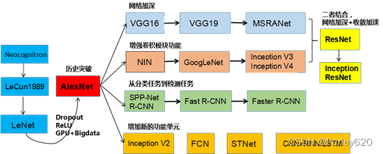
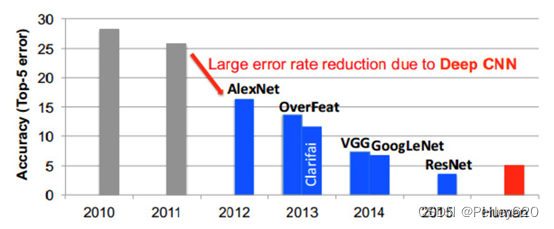
神经网络的进化
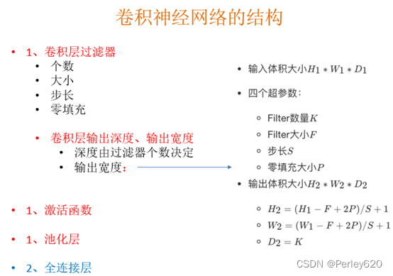
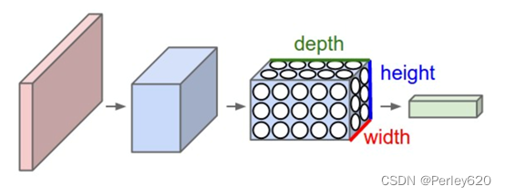
神经网络(neural networks)的基本组成包括输入层、隐藏层、输出层。而卷积神经网络的特点在于隐藏层分为卷积层和池化层(pooling layer,又叫下采样层)。
- 卷积层:通过在原始图像上平移来提取特征,每一个特征就是一个特征映射
- 池化层:通过特征后稀疏参数来减少学习的参数,降低网络的复杂度,(最大池化和平均池化)
结构示意图
零填充:
• 卷积核在提取特征映射时的动作称之为padding(零填充),由于移动步长不一定能整除整张图的像素宽度。其中有两种方式,SAME和VALID
- SAME:越过边缘取样,取样的面积和输入图像的像素宽度一致。
- VALID:不越过边缘取样,取样的面积小于输入人的图像的像素宽度
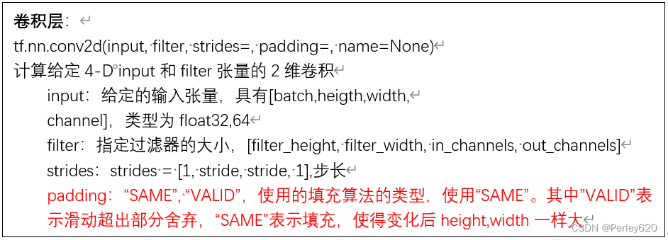
卷积层
tf.nn.conv2d(input, filter, strides=, padding=, name=None)
计算给定4-D input和filter张量的2维卷积
input:给定的输入张量,具有[batch,heigth,width,
channel],类型为float32,64
filter:指定过滤器的大小,[filter_height, filter_width, in_channels, out_channels]
strides:strides = [1, stride, stride, 1],步长
padding:“SAME”, “VALID”,使用的填充算法的类型,使用“SAME”。其中”VALID”表示滑动超出部分舍弃,“SAME”表示填充,使得变化后height,width一样大
新的激活函数-Relu
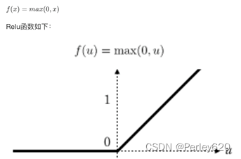
第一,采用sigmoid等函数,反向传播求误差梯度时,计算量相对大,而采用Relu激活函数,整个过程的计算量节省很多
第二,对于深层网络,sigmoid函数反向传播时,很容易就会出现梯度消失的情况(求不出权重和偏置)
激活函数:
tf.nn.relu(features, name=None)
features:卷积后加上偏置的结果
return:结果
池化层(Pooling)计算
Pooling层主要的作用是特征提取,通过去掉Feature Map中不重要的样本,进一步减少参数数量。Pooling的方法很多,最常用的是Max Pooling。
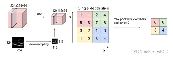
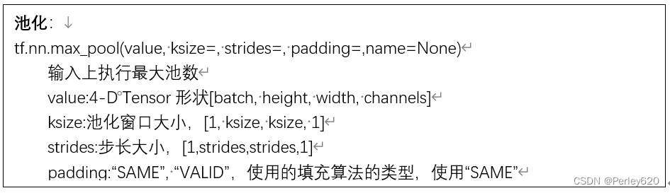
池化:
tf.nn.max_pool(value, ksize=, strides=, padding=,name=None)
输入上执行最大池数
value:4-D Tensor形状[batch, height, width, channels]
ksize:池化窗口大小,[1, ksize, ksize, 1]
strides:步长大小,[1,strides,strides,1]
padding:“SAME”, “VALID”,使用的填充算法的类型,使用“SAME”
Full Connected层:
分析:前面的卷积和池化相当于做特征工程,后面的全连接相当于做特征加权。最后的全连接层在整个卷积神经网络中起到“分类器”的作用。
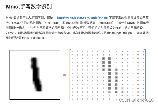
案例:Mnist手写数字图片识别卷积网络案例
流程:
1、准备数据
2、卷积、激活、池化(两层)
3、全连接层
4、计算准确率
import tensorflow as tf
old_v = tf.logging.get_verbosity()
tf.logging.set_verbosity(tf.logging.ERROR)
from tensorflow.examples.tutorials.mnist import input_data
# 定义一个初始化权重的函数
def weight_variable(shape):
    w = tf.Variable(tf.random_normal(shape=shape,mean=0.0,stddev=1.0))
    return w
# 定义一个初始化偏置的函数
def bias_variable(shape):
    b = tf.Variable(tf.constant(0.0,shape=shape))
    return b
def model():
    '''
    自定义的卷积模型
    :return:
    '''
    # 1、准备数据的占位符  x [None, 784]    y_true [None, 10]
    with tf.variable_scope("data"): # 作用域
        x = tf.placeholder(tf.float32, [None, 784])
        y_true = tf.placeholder(tf.int32, [None, 10])

    # 2、一卷积层 卷积 5x5x1,32个,strides=1
            ##   激活 tf.nn.relu,池化
    with tf.variable_scope("conv1"):  # 作用域
        # 随机初始化权重,偏置
        w_conv1 = weight_variable([5,5,1,32])
        b_conv1 = bias_variable([32])
        # 对 x进行形状的改变 [none,784]  ---> [none,28,28,1]
        x_reshape = tf.reshape(x,[-1,28,28,1])

        # 卷积 [none,28,28,1] ---> [none,28,28,32]
        x_relu = tf.nn.relu(tf.nn.conv2d(x_reshape,w_conv1,strides=[1,1,1,1],padding="SAME") + b_conv1)
        # 池化 2x2,strides=2,[none,28,28,32]---> [none,14,14,32]
        x_pool1 = tf.nn.max_pool(x_relu, ksize=[1,2,2,1],strides=[1,2,2,1], padding="SAME")

    # 3、二卷积层       卷积 5x5x32,64个,strides=1
    #             ##   激活 tf.nn.relu,池化
        # 随机初始化权重[5, 5, 32, 64],偏置
        w_conv2 = weight_variable([5, 5, 32, 64])
        b_conv2 = bias_variable([64])
        # 卷积,激活,池化计算
        # [none,14,14,32] ---> [none,14,14,64]
        x_relu2 = tf.nn.relu(tf.nn.conv2d(x_pool1, w_conv2, strides=[1, 1, 1, 1], padding="SAME") + b_conv2)
        # 池化 2x2,strides=2,[none,14,14,64]---> [none,7,7,64]
        x_pool2 = tf.nn.max_pool(x_relu2, ksize=[1, 2, 2, 1], strides=[1, 2, 2, 1], padding="SAME")

    # 4、全连接层 [none,7,7,64]---> [none,7*7*64]*[7*7*64,10] +[10] = [none,10]
    with tf.variable_scope("conv2"):  # 作用域none,
        # 随机初始化权重,偏置
        w_fc = weight_variable([7*7*64, 10])
        b_fc = bias_variable([10])

        # 修改形状 [none,7,7,64]---> [none,7*7*64],四维到二维
        x_fc_reshape = tf.reshape(x_pool2,[-1,7*7*64])

        # 矩阵运算得出每个样本的10个结果
        y_predict = tf.matmul(x_fc_reshape, w_fc) + b_fc

    return  x , y_true ,y_predict

def conv_fc():
    #获取真实数据
    mnist = input_data.read_data_sets("./data/mnist/", one_hot=True)
    # 定义模型,得出输出
    x, y_true, y_predict = model()

    # 进行交叉熵损失计算
    with tf.variable_scope("soft_cross"):
        # 求平均交叉熵损失
        loss = tf.reduce_mean(tf.nn.softmax_cross_entropy_with_logits(labels=y_true, logits=y_predict))

    # 4、梯度下降求出损失 学习率要比较小
    with tf.variable_scope("optimizer"):
        train_op = tf.train.GradientDescentOptimizer(0.0001).minimize(loss)# 学习率和最小化损失

    # 5、计算准确率
    with tf.variable_scope("acc"):
        equal_list = tf.equal(tf.argmax(y_true, 1), tf.argmax(y_predict, 1))
        # equal_list  None个样本   [1, 0, 1, 0, 1, 1,..........]
        accuracy = tf.reduce_mean(tf.cast(equal_list, tf.float32))

    # 定义一个初始化变量 op
    init_op = tf.global_variables_initializer()
    # 开启会话去训练

    with tf.Session() as sess:
        # 初始化变量
        sess.run(init_op)
        # 循环训练
        for i in range(1000):
            # 取出真实存在的特征值和目标值
            mnist_x, mnist_y = mnist.train.next_batch(50)
            # 运行train_op训练
            sess.run(train_op, feed_dict={x: mnist_x, y_true: mnist_y})
            print("训练第%d步,准确率为:%f" % (i, sess.run(accuracy, feed_dict={x: mnist_x, y_true: mnist_y})))
    return None

if __name__ == "__main__":
    conv_fc()
GoogleNet:


 748
748


 被折叠的 条评论
为什么被折叠?
被折叠的 条评论
为什么被折叠?
 到【灌水乐园】发言


