第二章——用Python实现感知器模型（MNIST数据集）

    感知机是1957年由Rosenblatt提出，是神经网络与支持向量机的基础，是二类分类的线性分类模型。

感知器模型

     适用问题：二类分类

     模型特点：分离超平面

     模型类型：判别模型

感知机学习策略

     学习策略：极小化误分点到超平面距离   

     学习的损失函数：误分点超平面距离

感知机学习算法

     学习算法：随机梯度下降

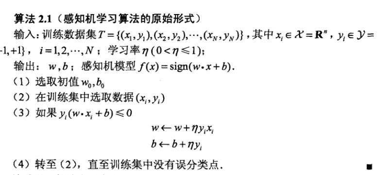
算法中感知器模型是一个sigmoid函数，于是上述模型是一个二分类的线性分类器。

数据集介绍

我们选择MNIST数据集进行实验

MNIST是一个入门级的计算机视觉数据集，它包含各种手写数字图片：

它也包含每一张图片对应的标签，告诉我们这个是数字几。比如，上面这四张图片的标签分别是5，0，4，1。

其官方下载地址：http://yann.lecun.com/exdb/mnist/

但是原始数据太麻烦了，我们选择kaggle提供的已处理好的数据
地址：https://www.kaggle.com/c/digit-recognizer/data

由于我们是二分类器，所以需要对train.csv中的label列进行一些微调，label等于0的继续等于0，label大于0改为1。

这样就将十分类的数据改为二分类的数据。
也可以从我的github上下载：https://github.com/WenDesi/lihang_book_algorithm/blob/master/data/train_binary.csv

HOG特征提取

MNIST数据都是28*28的图片，可选择的特征有很多，包括：
1. 自己提取特征
2. 将整个图片作为特征向量
3. HOG特征

我们选择HOG特征，HOG特征相关内容大家可以参考zouxy09 的相关博文

我们的目标是实用！因此只展示如何用Python提取HOG特征。

Python提取特征需要调用opencv2，代码如下所示

hog = cv2.HOGDescriptor('../hog.xml')
img = np.reshape(img,(28,28))
cv_img = img.astype(np.uint8)
hog_feature = hog.compute(cv_img)

其中hog.xml保存hog的配置信息，如下所示

<?xml version="1.0"?>
<opencv_storage>
<hog type_id="opencv-object-detector-hog">
  <winSize>
    28 28</winSize>
  <blockSize>
    14 14</blockSize>
  <blockStride>
    7 7</blockStride>
  <cellSize>
    7 7</cellSize>
  <nbins>9</nbins>
  <derivAperture>1</derivAperture>
  <winSigma>4.</winSigma>
  <histogramNormType>0</histogramNormType>
  <L2HysThreshold>2.0000000000000001e-001</L2HysThreshold>
  <gammaCorrection>1</gammaCorrection>
  <nlevels>64</nlevels></hog>
</opencv_storage>

关于更多hog特征配置信息，大家可以参考这篇文章

代码

代码我已经放到Github上了，大家可以参考我的Github:https://github.com/WenDesi/lihang_book_algorithm

感知器代码位于perceptron/binary_perceptron.py

这里也贴一下代码

#encoding=utf-8

import pandas as pd
import numpy as np
import cv2
import random
import time

from sklearn.cross_validation import train_test_split
from sklearn.metrics import accuracy_score

# 利用opencv获取图像hog特征
def get_hog_features(trainset):
    features = []

    hog = cv2.HOGDescriptor('../hog.xml')

    for img in trainset:
        img = np.reshape(img,(28,28))
        cv_img = img.astype(np.uint8)

        hog_feature = hog.compute(cv_img)
        # hog_feature = np.transpose(hog_feature)
        features.append(hog_feature)

    features = np.array(features)
    features = np.reshape(features,(-1,324))

    return features

def Train(trainset,train_labels):
    # 获取参数
    trainset_size = len(train_labels)

    # 初始化 w,b
    w = np.zeros((feature_length,1))
    b = 0

    study_count = 0                         # 学习次数记录，只有当分类错误时才会增加
    nochange_count = 0                      # 统计连续分类正确数，当分类错误时归为0
    nochange_upper_limit = 100000           # 连续分类正确上界，当连续分类超过上界时，认为已训练好，退出训练

    while True:
        nochange_count += 1
        if nochange_count > nochange_upper_limit:
            break

        # 随机选的数据
        index = random.randint(0,trainset_size-1)
        img = trainset[index]
        label = train_labels[index]

        # 计算yi(w*xi+b)
        yi = int(label != object_num) * 2 - 1                       # 如果等于object_num, yi= 1, 否则yi=1
        result = yi * (np.dot(img,w) + b)

        # 如果yi(w*xi+b) <= 0 则更新 w 与 b 的值
        if result <= 0:
            img = np.reshape(trainset[index],(feature_length,1))    # 为了维数统一，需重新设定一下维度

            w += img*yi*study_step                                  # 按算法步骤3更新参数
            b += yi*study_step

            study_count += 1
            if study_count > study_total:
                break
            nochange_count = 0
    return w,b

def Predict(testset,w,b ):
    predict = []
    for img in testset:
        result = np.dot(img,w) + b
        result = result > 0
        predict.append(result)
    return np.array(predict)

study_step = 0.0001                                 # 学习步长
study_total = 10000                                 # 学习次数
feature_length = 324                                # hog特征维度
object_num = 0                                      # 分类的数字

if __name__ == '__main__':

    print 'Start read data'

    time_1 = time.time()

    raw_data = pd.read_csv('../data/train_binary.csv',header=0)
    data = raw_data.values

    imgs = data[0::,1::]
    labels = data[::,0]

    features = get_hog_features(imgs)

    # 选取 2/3 数据作为训练集， 1/3 数据作为测试集
    train_features, test_features, train_labels, test_labels = train_test_split(features, labels, test_size=0.33, random_state=23323)
    # print train_features.shape
    # print train_features.shape

    time_2 = time.time()
    print 'read data cost ',time_2 - time_1,' second','\n'

    print 'Start training'
    w,b = Train(train_features,train_labels)
    time_3 = time.time()
    print 'training cost ',time_3 - time_2,' second','\n'

    print 'Start predicting'
    test_predict = Predict(test_features,w,b)
    time_4 = time.time()
    print 'predicting cost ',time_4 - time_3,' second','\n'

    score = accuracy_score(test_labels,test_predict)
    print "The accruacy socre is ", score

运行结果如下所示，可以看到准确度还不错

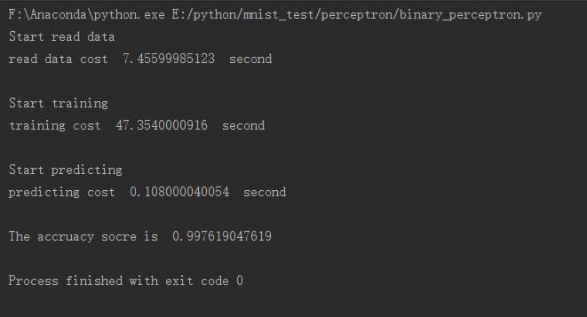
算法的收敛性

      证明：Novikoff定理

算法的对偶形式

      为了求解更简单，所以用对偶形式