如何使用 基于连续小波变换时频图的CNN轴承故障诊断模型 Python、jupyter notebook，实现训练评估及可视化

基于连续小波变换时频图的CNN轴承故障诊断模型
Python、jupyter notebook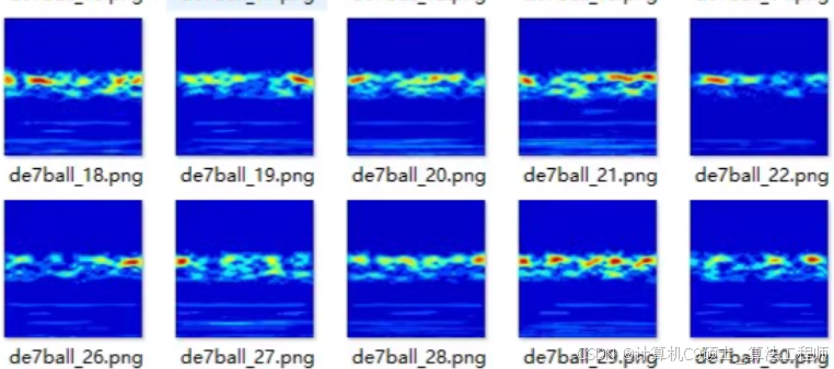

使用基于连续小波变换（Continuous Wavelet Transform, CWT）生成的时频图来构建一个卷积神经网络（CNN）模型进行滚动轴承故障诊断。以下是详细的步骤和代码示例。

步骤概述

1. 数据集准备
2. 特征提取（CWT时频图）
3. 数据预处理
4. 构建CNN模型
5. 模型训练
6. 模型评估
7. 结果可视化

详细步骤

1. 数据集准备

确保你的数据集已经按照上述格式准备好，并且包含相应的文件目录结构。

bearing_datasets/
├── CWRU/
│   ├── normal.mat
│   ├── inner_race_fault.mat
│   └── ...
├── XJTU/
│   ├── normal.mat
│   ├── ball_fault.mat
│   └── ...
├── Jiangnan/
│   ├── normal.csv
│   ├── outer_race_fault.csv
│   └── ...
└── Southeast/
    ├── normal.csv
    ├── inner_race_fault.csv
    └── ...

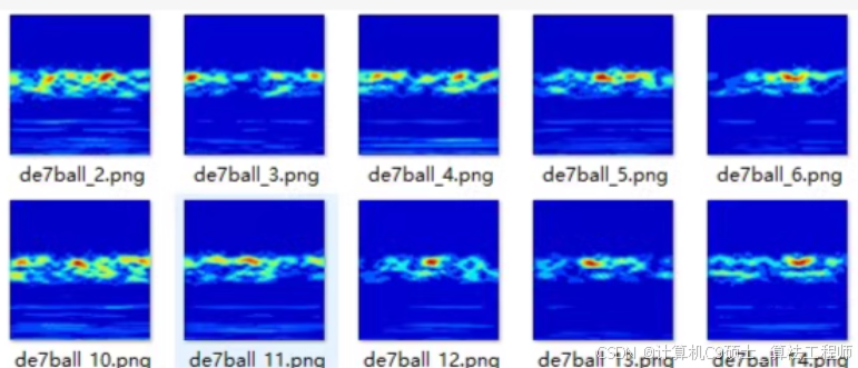
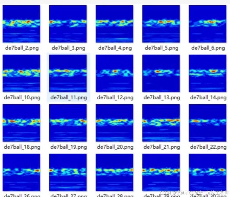
2. 特征提取（CWT时频图）

使用PyWavelets库来计算连续小波变换并生成时频图。

import os
import numpy as np
import pandas as pd
import scipy.io as sio
from pywt import cwt, Morlet
import matplotlib.pyplot as plt
from sklearn.preprocessing import StandardScaler, LabelEncoder
from sklearn.model_selection import train_test_split
from tensorflow.keras.models import Sequential
from tensorflow.keras.layers import Conv2D, MaxPooling2D, Flatten, Dense, Dropout
from tensorflow.keras.utils import to_categorical
from tensorflow.keras.callbacks import EarlyStopping

# Step 1: Data Preparation
# Ensure your dataset is organized as described above.

# Step 2: Feature Extraction (CWT Time-Frequency Maps)
def compute_cwt(signal, scales, wavelet='morl', sampling_period=1):
    coefficients, frequencies = cwt(signal, scales, wavelet, sampling_period=sampling_period)
    return coefficients

def load_and_extract_features(dataset_path, fs=12000):
    features = []
    labels = []
    
    scales = np.arange(1, 128)  # Define the range of scales for CWT
    
    for filename in os.listdir(dataset_path):
        if filename.endswith('.mat'):
            data = sio.loadmat(os.path.join(dataset_path, filename))
            signal = data[list(data.keys())[-1]].flatten()
            label = filename.split('_')[0]  # Assuming label is part of the filename
            cwt_map = compute_cwt(signal, scales, sampling_period=1/fs)
            features.append(cwt_map)
            labels.append(label)
        elif filename.endswith('.csv'):
            data = pd.read_csv(os.path.join(dataset_path, filename))
            signal = data.iloc[:, 0].values
            label = filename.split('_')[0]  # Assuming label is part of the filename
            cwt_map = compute_cwt(signal, scales, sampling_period=1/fs)
            features.append(cwt_map)
            labels.append(label)
    
    return np.array(features), np.array(labels)

# Load and extract features from each dataset
cwru_features, cwru_labels = load_and_extract_features('bearing_datasets/CWRU')
xjtu_features, xjtu_labels = load_and_extract_features('bearing_datasets/XJTU')
jiangnan_features, jiangnan_labels = load_and_extract_features('bearing_datasets/Jiangnan')
southeast_features, southeast_labels = load_and_extract_features('bearing_datasets/Southeast')

# Combine all datasets
all_features = np.vstack((cwru_features, xjtu_features, jiangnan_features, southeast_features))
all_labels = np.concatenate((cwru_labels, xjtu_labels, jiangnan_labels, southeast_labels))

# Normalize features
all_features_normalized = (all_features - np.min(all_features)) / (np.max(all_features) - np.min(all_features))

3. 数据预处理

标准化特征数据并划分训练集和测试集。

# Encode labels
label_encoder = LabelEncoder()
all_labels_encoded = label_encoder.fit_transform(all_labels)

# Reshape features to include channel dimension
all_features_reshaped = all_features_normalized[..., np.newaxis]

# Split into training and testing sets
X_train, X_test, y_train, y_test = train_test_split(all_features_reshaped, all_labels_encoded, test_size=0.2, random_state=42)

# Convert labels to categorical one-hot encoding
y_train_categorical = to_categorical(y_train)
y_test_categorical = to_categorical(y_test)

4. 构建CNN模型

使用Keras构建一个简单的CNN模型。

# Build CNN model
model = Sequential([
    Conv2D(32, kernel_size=(3, 3), activation='relu', input_shape=X_train.shape[1:]),
    MaxPooling2D(pool_size=(2, 2)),
    Dropout(0.25),
    Conv2D(64, kernel_size=(3, 3), activation='relu'),
    MaxPooling2D(pool_size=(2, 2)),
    Dropout(0.25),
    Flatten(),
    Dense(128, activation='relu'),
    Dropout(0.5),
    Dense(len(np.unique(all_labels_encoded)), activation='softmax')
])

# Compile the model
model.compile(optimizer='adam', loss='categorical_crossentropy', metrics=['accuracy'])

# Print model summary
model.summary()

5. 模型训练

训练CNN模型。

# Define early stopping callback
early_stopping = EarlyStopping(monitor='val_loss', patience=10, restore_best_weights=True)

# Train the model
history = model.fit(X_train, y_train_categorical, validation_data=(X_test, y_test_categorical), epochs=100, batch_size=32, callbacks=[early_stopping])

6. 模型评估

评估模型性能。

# Evaluate the model
test_loss, test_accuracy = model.evaluate(X_test, y_test_categorical)
print(f"Test Accuracy: {test_accuracy:.4f}")

# Plot training & validation accuracy values
plt.figure(figsize=(12, 4))
plt.subplot(1, 2, 1)
plt.plot(history.history['accuracy'])
plt.plot(history.history['val_accuracy'])
plt.title('Model accuracy')
plt.ylabel('Accuracy')
plt.xlabel('Epoch')
plt.legend(['Train', 'Validation'], loc='upper left')

# Plot training & validation loss values
plt.subplot(1, 2, 2)
plt.plot(history.history['loss'])
plt.plot(history.history['val_loss'])
plt.title('Model loss')
plt.ylabel('Loss')
plt.xlabel('Epoch')
plt.legend(['Train', 'Validation'], loc='upper left')

plt.show()

7. 结果可视化

可视化预测结果。

# Predict on test set
y_pred = model.predict(X_test)
y_pred_classes = np.argmax(y_pred, axis=1)

# Confusion matrix
from sklearn.metrics import confusion_matrix, classification_report
import seaborn as sns

conf_matrix = confusion_matrix(y_test, y_pred_classes)
sns.heatmap(conf_matrix, annot=True, fmt='d', cmap='Blues', xticklabels=label_encoder.classes_, yticklabels=label_encoder.classes_)
plt.title('Confusion Matrix')
plt.xlabel('Predicted')
plt.ylabel('True')
plt.xticks(rotation=90)
plt.yticks(rotation=0)
plt.show()

# Classification report
print("Classification Report:")
print(classification_report(y_test, y_pred_classes, target_names=label_encoder.classes_))

完整代码

以下是完整的代码示例，包含了从数据加载、特征提取、数据预处理、模型训练到结果对比的所有步骤。

运行脚本

在终端中运行以下命令来执行整个流程：

python main.py

总结

以上文档包含了从数据集准备、特征提取（CWT时频图）、数据预处理、模型训练与评估、可视化结果到结果对比的所有步骤。希望这些详细的信息和代码能够帮助你顺利实施和优化你的滚动轴承故障诊断系统。