


首先用R语言构造数据点
> y <- c(5, 7, 9, 11, 16, 20)
> x <- c(1, 2, 3, 4, 7, 9)
> plot(x,y)
绘制的散点图图像如下所示
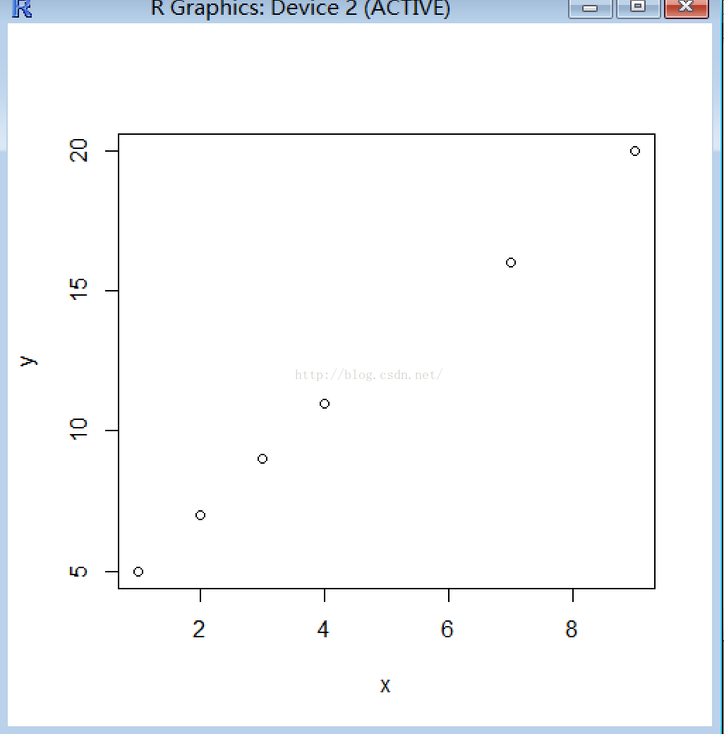
> y <- c(5, 7, 9, 11, 16, 20)
> x <- c(1, 2, 3, 4, 7, 9)
> plot(x,y) 2226
2226

 被折叠的 条评论
为什么被折叠?
被折叠的 条评论
为什么被折叠?
 到【灌水乐园】发言


 最低0.47元/天 解锁文章


