Computer Vision Source Code

http://clickdamage.com/sourcecode/index.php

Computer Vision Source Code

CLICKDAMAGE

Please report code bugs etc to:oconaire [at-symbol] gmail [dot] com 

Matlab code for Skin Detection:  Info: Readme.TXT  Full Matlab code and demo: skindetector.zip  If you publish work which uses this code, please reference: Ciarán Ó Conaire, Noel E. O'Connor and Alan F. Smeaton, "Detector adaptation by maximising agreement between independent data sources", IEEE International Workshop on Object Tracking and Classification Beyond the Visible Spectrum 2007  (1) (2) (3)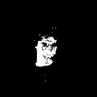  (1) Original image, (2) Skin Likelihood image and (3) Detected Skin (using a threshold of zero)

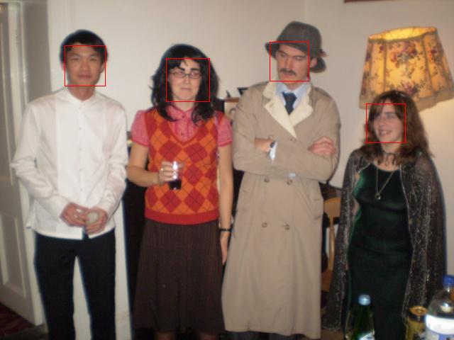
Command line Face Detection This uses the face-detector in the Blepo computer vision library, which in turn uses the OpenCV implementation of the Viola-Jones face detection method.  Info and usage: README  Source code only (requires Blepo): FaceDetect.cpp (Windows) Executable only (does not require Blepo): *BROKEN*(sorry) FaceDetector.ZIP

Simple MATLAB scripts These small scripts are required for some of the other code on this page to work.  Code: makelinear.m - convert any size array/matrix into a Nx1 vector, where N = prod(size(inputMatrix))  Code: shownormimage.m - display any single-band or triple-band image, by normalising each band it so that the darkest pixel is black and the brightest is white  Code: filter3.m - uses filter2 to perform filtering on each image band separately  Code: removezeros.m - removes zero values from a vector.  Code: integrate.m - compute the cumulative sum of values in the rows of a matrix.

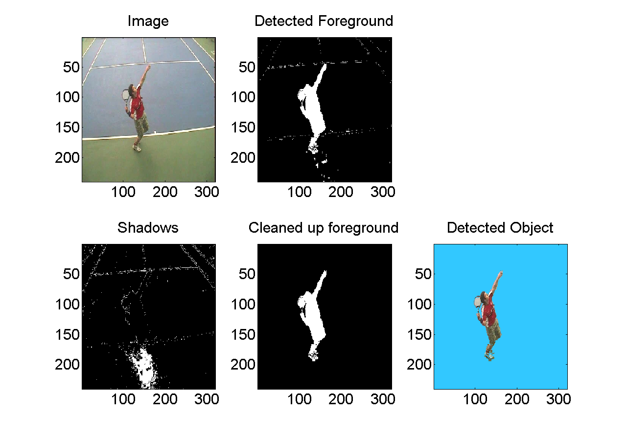
Layered Background Model  Reference: Performance analysis and visualisation in tennis using a low-cost camera network, Philip Kelly, Ciarán Ó Conaire, David Monaghan, Jogile Kuklyte, Damien Connaghan, Juan Diego Pérez-Moneo Agapito, Petros Daras, Multimedia Grand Challenge Track at ACM Multimedia 2010, 25-29 October 2010, Firenze, Italy.  PDF Version  Download Code: layered_background_model_code.zip  Usage: model creation: N = 5; % number of layers T = 20; % RGB Euclidian threshold (for determining if the pixel matches a layer) U = 0.999; % update rate A = 0.85; % fraction of observed colour to account for in the background im = imread('image.jpg'); bgmodel = initLayeredBackgroundModel(im, N, T, U, A); model updating: im = imread('image_new.jpg'); [bgmodel, foreground, bridif, coldif, shadows] = updateLayeredBackgroundModel(bgmodel, im); returns: updated background model foreground image brightness difference colour difference shadow pixels image

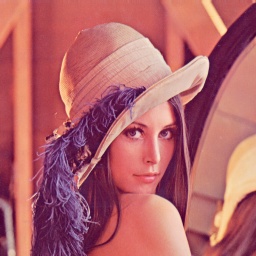
Filtering/Image blurring Code: gaussianFilter.m  Example:  % setup filter filt = gaussianFilter(31,5); % read in an image im = double(imread('lena.jpg')); % filter image imf = filter3(filt, im); % show images (get the code for 'shownormimage.m'/'filter3.m' above) shownormimage(im); pause shownormimage(imf); pause

Adaptive Image Thresholding The following pieces of code implement the adaptive thresholding methods of Otsu, Kapur and Rosin.  References to the original papers given below.  Code: otsuThreshold.m  Code: kapurThreshold.m  Code: rosinThreshold.m  Code: dootsuthreshold.m  Code: dokapurthreshold.m  Code: dorosinthreshold.m  Example usage: % read in image 0000 of an image sequence im1 = double(imread('image0000.jpg')); % read in image 0025 of an image sequence im2 = double(imread('image0025.jpg')); % compute the difference image (Euclidian distance in RGB space) dif = sqrt(sum((im1-im2).^2,3)); % compute difference image histogram [h, hc] = hist(makelinear(dif), 256); % perform thresholding to detect motion To = hc(otsuThreshold(h)); Tk = hc(kapurThreshold(h)); Tr = hc(rosinThreshold(h)); % display results shownormimage(dif >= To); title('Otsu result'); pause shownormimage(dif >= Tk); title('Kapur result'); pause shownormimage(dif >= Tr); title('Rosin result'); pause % Alternatively, you can use % shownormimage(dokapurthreshold(dif)); % .... 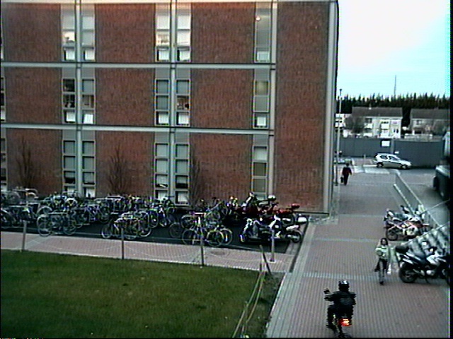etc  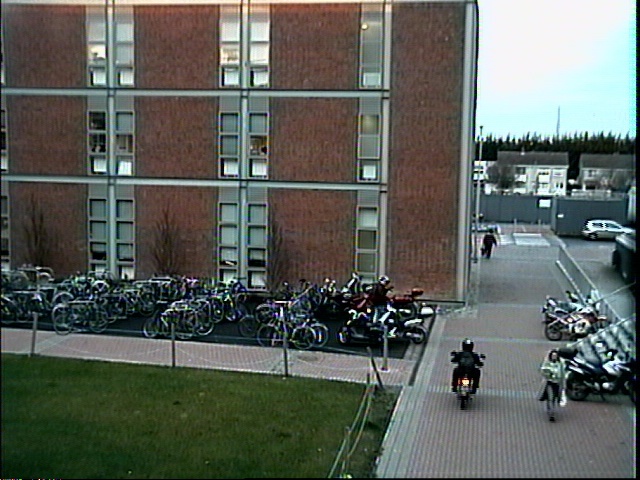  Source images (above) 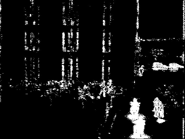 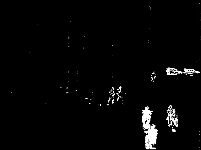 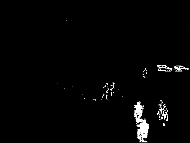   Thresholded difference images (from left to right): Rosin, Kapur and Otsu's method.  References: N. Otsu, A threshold selection method from gray-level histogram, IEEE Trans on System Man Cybernetics 9 (1979), no. 1, 62-66. J. Kapur, P. Sahoo, and A. Wong, A new method for graylevel picture thresholding using the entropy of the histogram, Computer Graphics and Image Processing 29 (1985), no. 3, 273-285 P. L. Rosin, Unimodal thresholding, Pattern Recognition 34 (2001), no. 11, 2083-2096

Image Descriptors and Image Similarity Code to extract global descriptors for images and to compare these descriptors.  Can be used for image retrieval, tracking, etc.  Image colour histogram extraction: getPatchHist.m  Histogram comparison using the Bhattacharyya coefficient: compareHists.m  Image colour spatiogram extraction: getPatchSpatiogram_fast.m  Spatiogram comparison: compareSpatiograms_new_fast.m  MPEG-7 Edge Orientation Histogram extraction: edgeOrientationHistogram.m  (Note: code for histogram comparison can be used with both colour histograms and edge orientation histograms)  Sample code: % ---- Code to compare image histograms ---- % read in database image im1 = double(imread('flower.jpg')); % read in query image im2 = double(imread('garden.jpg')); % Both images are RGB Colour images % Extract an 8x8x8 colour histogram from each image bins = 8; h1 = getPatchHist(im1, bins); h2 = getPatchHist(im2, bins); % compare their histograms using the Bhattacharyya coefficient sim = compareHists(h1,h2); % 0 = very low similarity % 0.9 = good similarity % 1 = perfect similarity disp(sprintf('Image histogram similarity = %f', sim)); % ---- Code to compare image SPATIOGRAMS ---- % Both images are RGB Colour images % Extract an 8x8x8 colour SPATIOGRAM from each image bins = 8; [h1,mu1,sigma1] = getPatchSpatiogram_fast(im1, bins); [h2,mu2,sigma2] = getPatchSpatiogram_fast(im2, bins); % compare their histograms using the Bhattacharyya coefficient sim = compareSpatiograms_new_fast(h1,mu1,sigma1,h2,mu2,sigma2); % 0 = very low similarity % 0.9 = good similarity % 1 = perfect similarity disp(sprintf('Image spatiogram similarity = %f', sim));

Nearest-Neighbour search using KD-Trees (coming soon...)

Hierarchical Clustering using K-means Finding the nearest neighbour of a data point in high-dimensional space is known to be a hard problem [1]. This code clusters the data into a hierarchy of clusters and does a depth-first search to find the approximate nearest-neighbour to the query point. This technique was used in [2] to match 128-dimensional SIFT descriptors to their visual words.  K-means clustering: kmeans.m Building a hierarchical tree of D-dimensional points: kmeanshierarchy.m Approximate Nearest-Neighbour using a hierarchical tree: kmeanshierarchy_findpoint.m  Sample code: D=2; % dimensionality K=2; % branching factor N=50; % size of each dataset iters = 3; % number of clustering iterations % setup datasets, first column is the ID dataset1 = [ones(N,1) randn(N,D)]; dataset2 = [2*ones(N,1) 2*randn(N,2)+repmat([-5 3],[N 1])]; dataset3 = [3*ones(N,1) 1.5*randn(N,2)+repmat([5 3],[N 1])]; data = [dataset1; dataset2; dataset3]; % build the tree structure % select columns 2 to D+1, column 1 stores the dataset-ID that the point came from. [hierarchy] = kmeanshierarchy(data, 2, D+1, iters, K); for test = 1:16 % Generate a random point point = [rand*16-8 randn(1,D-1)]; % plot the data cols = ['bo';'rx';'gv']; hold off for i = 1:size(data,1) plot(data(i,2),data(i,3),cols(data(i,1),:)); hold on end hold off if (test==1) title('Data Clusters (1=Blue, 2=Red, 3=Green)') pause end hold on plot(point(1), point(2), 'ks'); hold off title('New Point (shown as a black square)'); pause % Find its approximate nearest-neighbour in the tree nn = kmeanshierarchy_findpoint(point, hierarchy, 2, D+1, K); nearest_neighbour = nn(2:(D+1)); % Which set did it come from? set_id = nn(1); line([point(1) nearest_neighbour(1)],[point(2) nearest_neighbour(2)]) title(sprintf('Approx Nearest Neighbour: Set %d', set_id)) pause end [1] Piotr Indyk. Nearest neighbors in high-dimensional spaces. Handbook of Discrete and Computational Geometry, chapter 39.  Editors: Jacob E. Goodman and Joseph O'Rourke, CRC Press, 2nd edition, 2004. CITESEER LINK  [2] David Nistér and Henrik Stewenius, Scalable Recognition with a Vocabulary Tree, CVPR'06 CITESEER LINK

Mutual Information Thresholding The idea of selecting thresholds for data "adaptively" has been around for a long time. The standard paradigm is to observe some property of the data (such as histogram shape, entropy, spatial layout, etc) and to choose a threshold that maximises some proposed performance measure. Mutual Information (MI) Thresholding takes a different approach. Instead of examining a single property of the data, it looks instead at how choices of threshold for two sources of data will affect how well they "agree" with each other.  More formally: Given two sources of data that have uncorrelated noise, choose a threshold for each of the sources, such that the mutual information between the resulting binary signals is maximised. This search through threshold-space can be done very efficiently using integral-images.  Matlab Code Download: ZIP FILE  Sample code: N=100; signal = 30; noise = 5; im = zeros(N,N); im(round(N/3:N/2),round(N/3:N/2)) = signal; im1 = abs(im + noise * randn(N,N)); im2 = abs(im + 1.5*noise * randn(N,N)); [T1, T2, mi, imT1, imT2, imF, quality, miscore, mii1, mii2] = mutualinfoThreshold(im1, im2); subplot(1,2,1); shownormimage2(im1); subplot(1,2,2); shownormimage2(im2); pause subplot(1,2,1); shownormimage2(imT1); title(sprintf('Threshold = %f', T1)); subplot(1,2,2); shownormimage2(imT2); title(sprintf('Threshold = %f', T2)); pause subplot(1,1,1); shownormimage2(mi); title('Mutual Information Surface'); pause References: C. Ó Conaire, N. O'Connor, E. Cooke and A. Smeaton, Detection Thresholding using Mutual Information, VISAPP 2006 PDF Available C. Ó Conaire and N. O'Connor, Unsupervised feature selection for detection using mutual information thresholding, WIAMIS 2008