


深度学习基础学习——PyTorch实现VGG网络
目录:
- 概要描述
- 实验结果
- 代码示例
- 运行示例
- 问题报错及解决
- 论文重点内容学习
- 参考文献
一、概要描述
- VGG网络的亮点:堆叠多个3X3卷积核来替代大尺度卷积核(减少所需参数)
- 堆叠2个3X3的卷积核替代5X5的卷积核,堆叠3个3X3的卷积核替代7X7的卷积核,拥有相同的感受野
- 感受野(Receptive Field):决定某一层输出结果中一个元素所对应的输入层的区域大小,即输出特征矩阵上的一个单元对应输入层上的区域大小
- 计算公式:out = (in - F + 2P) / S +1,其中F为卷积核大小,P为Padding大小,S为Stride
- conv:stride为1,padding为1
- maxpool:size为2,stride为2
- 感受野计算公式:F(i) = (F(i + 1) - 1) X Stride + Ksize,其中F(i)为第i层感受野,Stride为第i层步距,Ksize为卷积核或池化核尺寸
- 假设特征矩阵Feature map:F(3) = 1,
- Pool1:Size:2X2,Stride:2,F(2) = (F(3) - 1) X 2 + 2 = 2
- Conv1:Size:3X3,Stride:2,F(1) = (F(2) - 1) X 2 + 3 = 5
- 即通过3X3卷积及池化后所得到的特征矩阵上的一个单位,在原图中对应的感受野是5X5的大小
- 堆叠3个3X3的卷积核替代7X7的卷积核,推导:
- 假设特征矩阵Feature map:F(4) = 1,
- Conv3X3(3):Size:3X3,Stride:1,F(3) = (F(4) - 1) X 1 + 3 = 3
- Conv3X3(2):Size:3X3,Stride:1,F(2) = (F(3) - 1) X 1 + 3 = 5
- Conv3X3(1):Size:3X3,Stride:1,F(1) = (F(2) - 1) X 1 + 3 = 7
- 即通过3层3X3的卷积核卷积后所得到的特征矩阵上的一个单位,在原图中对应的感受野是7X7的大小,和采用一个7X7的卷积核所得到的感受野是相同的。
- 使用7X7卷积核所需参数,与堆叠3个3X3的卷积核所需参数比较(假设输入输出Channel为C):
- 7X7XCXC = 49C²(第一个C为输入特征矩阵的深度,第二个C为卷积核的个数)
- 3X(3X3XCXC) = 27C²

二、实验结果
- 服务器:Ubuntu18.04
- Pytorch:1.2.0
- Python:3.7.9
- cuda:10.0
- GPU显卡:Nvida RTX2080Ti 两张(11GB / 张)
- 数据集:cifar-10

| method | layers | dataset | batch size | learning rate | epoch | dropout | top-1 accuracy | top-3 accuracy |
|---|---|---|---|---|---|---|---|---|
| vgg16 | [16, 16, 'M', 32, 32, 'M', 64, 64, 64, 'M', 128, 128, 128, 'M', 128, 128, 128, 'M', FC-50, FC-50, FC-10] | cifar-10 | 64 | 0.0001 | 20 | 50% | 56.0% | 84.0% |
| vgg16 | [16, 16, 'M', 32, 32, 'M', 64, 64, 64, 'M', 128, 128, 128, 'M', 128, 128, 128, 'M', FC-50, FC-50, FC-10] | cifar-10 | 64 | 0.0001 | 30 | 50% | 61.0% | 87.4% |
| vgg16 | [16, 16, 'M', 32, 32, 'M', 64, 64, 64, 'M', 128, 128, 128, 'M', 128, 128, 128, 'M', FC-50, FC-50, FC-10] | cifar-10 | 64 | 0.0001 | 30 | 40% | 62.0% | 87.0% |
| vgg16 | [16, 16, 'M', 32, 32, 'M', 64, 64, 64, 'M', 128, 128, 128, 'M', 128, 128, 128, 'M', FC-70, FC-70, FC-10] | cifar-10 | 64 | 0.0001 | 30 | 40% | 62.1% | 88.0% |
| vgg16 | [16, 16, 'M', 32, 32, 'M', 64, 64, 64, 'M', 128, 128, 128, 'M', 128, 128, 128, 'M', FC-256, FC-256, FC-10] | cifar-10 | 64 | 0.0001 | 30 | 40% | 65.3% | 89.9% |
| vgg16 | [16, 16, 'M', 32, 32, 'M', 64, 64, 64, 'M', 128, 128, 128, 'M', 128, 128, 128, 'M', FC-256, FC-256, FC-10] | cifar-10 | 32 | 0.0001 | 30 | 40% | 69.7% | 91.9% |
| vgg16 | [16, 16, 'M', 32, 32, 'M', 64, 64, 64, 'M', 128, 128, 128, 'M', 128, 128, 128, 'M', FC-256, FC-256, FC-10] | cifar-10 | 32 | 0.0001 | 30 | 50% | 67.2% | 90.4% |
| vgg16 | [16, 16, 'M', 32, 32, 'M', 64, 64, 64, 'M', 128, 128, 128, 'M', 128, 128, 128, 'M', FC-512, FC-512, FC-10] | cifar-10 | 32 | 0.0001 | 30 | 40% | 70.4% | 91.7% |
| vgg16 | [16, 16, 'M', 32, 32, 'M', 64, 64, 64, 'M', 128, 128, 128, 'M', 128, 128, 128, 'M', FC-512, FC-512, FC-10] | cifar-10 | 32 | 0.0001 | 50 | 40% | 75.5% | 93.2% |
结论:在实验过程中,因时间原因,通过配置不同的超参数,仅测试了9组,在最后采用如上表中红色标注的行所示,Top-1准确率为:75.49%,Top-5准确率为:93.22%

三、代码示例
(1)model.py
import torch.nn as nn
import torch

class VGG(nn.Module):
    def __init__(self, features, num_classes=10, init_weights=False):
        super(VGG, self).__init__()
        self.features = features
        # 三层全连接层
        self.classifier = nn.Sequential(
            nn.Dropout(p=0.4), # 40%的比例随机失活神经元,减少过拟合
            nn.Linear(128*1*1, 512), # 第一层全连接层,第一个参数为:输入结点个数,第二个参数为:展平处理以后得到一维向量的元素个数
            nn.ReLU(True),
            nn.Dropout(p=0.4),
            nn.Linear(512, 512),
            nn.ReLU(True),
            nn.Linear(512, num_classes)
        )
        if init_weights: # 是否需要参数初始化
            self._initialize_weights()

    def forward(self, x):
        x = self.features(x)
        x = torch.flatten(x, start_dim=1) # 展平处理,从第一个维度channel开始展平,因为第0个维度是batch维度
        x = self.classifier(x)
        return x

    def _initialize_weights(self):
        for m in self.modules():
            if isinstance(m, nn.Conv2d):
                # nn.init.kaiming_normal_(m.weight, mode='fan_out', nonlinearity='relu')
                '''
                    nn.init中实现的初始化函数:
                    uniform:均匀分布
                    normal:正态分布
                    constant:初始化为常数
                    Xavier:输入和输出的方差相同,包括正向和反向传播
                    He initialization:torch.nn.init.kaiming_uniform_和torch.nn.init.kaiming_normal_,针对RELU
                '''
                nn.init.xavier_uniform_(m.weight)
                if m.bias is not None:
                    nn.init.constant_(m.bias, 0) # 默认偏置初始化为0
            elif isinstance(m, nn.Linear):
                nn.init.xavier_uniform_(m.weight)
                # nn.init.normal_(m.weight, 0, 0.01)
                nn.init.constant_(m.bias, 0)

def make_features(cfg: list):
    layers = [] # 存放每一层结构
    in_channels = 3
    for v in cfg:
        if v == "M":
            layers += [nn.MaxPool2d(kernel_size=2, stride=2)]
        else:
            conv2d = nn.Conv2d(in_channels, v, kernel_size=3, padding=1)
            layers += [conv2d, nn.ReLU(True)]
            in_channels = v
    return nn.Sequential(*layers) #非关键字参数传入

# 定义字典数据类型cfgs
cfgs = {
    'vgg11': [64, 'M', 128, 'M', 256, 256, 'M', 512, 512, 'M', 512, 512, 'M'],
    'vgg13': [64, 64, 'M', 128, 128, 'M', 256, 256, 'M', 512, 512, 'M', 512, 512, 'M'],
    'vgg16-cifar10': [16, 16, 'M', 32, 32, 'M', 64, 64, 64, 'M', 128, 128, 128, 'M', 128, 128, 128, 'M'],
    'vgg19': [64, 64, 'M', 128, 128, 'M', 256, 256, 256, 256, 'M', 512, 512, 512, 512, 'M', 512, 512, 512, 512, 'M'],
}

def vgg(model_name, **kwargs):
    try:
        cfg = cfgs[model_name]
    except:
        print("Warning: model number {} not in cfgs dict!".format(model_name))
        exit(-1)
    model = VGG(make_features(cfg), **kwargs)
    print(model)
    return model
(2)train.py
import time
import sys
import torch.nn as nn
import torchvision
from torchvision import transforms
import torch.optim as optim # 实现各种优化算法的库
import torch
import matplotlib.pyplot as plt
from model import vgg
from opt import dealOpt
device = torch.device("cuda:0" if torch.cuda.is_available() else "cpu") # 表示起始cuda的device_id为0
torch.backends.cudnn.enabled = True
if __name__ == "__main__":
classNum, image_path, model_name, epochNum, lr = dealOpt(sys.argv[1:])
batch_size = 32
num_workers = 4
top_k = 3
"""
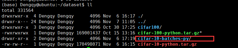
root:cifar-10-batches-py的根目录
train:为True是训练集,False是测试集
dowload:False从互联网上下载数据
"""
train_dataset = torchvision.datasets.CIFAR10(
root=image_path,
train=True,
transform=transforms.Compose([transforms.RandomResizedCrop(32), # 随机裁剪
transforms.RandomHorizontalFlip(), # 随机水平翻转
transforms.ToTensor(), # 转换成Tensor格式
transforms.Normalize(mean=(0.5, 0.5, 0.5), std=(0.5, 0.5, 0.5))]),# 标准化处理,channel=(channel - mean) / std,将每个值映射在[-1,1]
download=False
)
"""
数据加载器。组合数据集和采样器,并在数据集上提供单进程或多进程迭代器
shuffle:在每个epoch,对数据进行重新排序
num_workers:由多少个子进程来处理data loading
"""
train_loader = torch.utils.data.DataLoader(train_dataset, batch_size=batch_size, shuffle=True, num_workers=num_workers)
train_num = len(train_dataset)
test_dataset = torchvision.datasets.CIFAR10(
root=image_path,
train=False,
transform=transforms.Compose([transforms.Resize((32, 32)),
transforms.ToTensor(),
transforms.Normalize(mean=(0.5, 0.5, 0.5), std=(0.5, 0.5, 0.5))]),
download=False
)
test_loader = torch.utils.data.DataLoader(test_dataset, batch_size=batch_size, shuffle=False, num_workers=num_workers)
test_num = len(test_dataset)
print("train_dataset's num = %d, test_dataset's num = %d" %(train_num, test_num))
category_list = train_dataset.class_to_idx
cla_dict = dict((val, key) for key, val in category_list.items())
net = vgg(model_name=model_name, num_classes=classNum, init_weights=True)
if torch.cuda.device_count() > 1: # 采用多GPU训练
net = nn.DataParallel(net, device_ids=[0,1])
net.to(device)
loss_function = nn.CrossEntropyLoss() # 交叉熵损失函数用于多分类
optimizer = optim.Adam(net.parameters(), lr=0.0001) # Adam:基于梯度的优化算法
best_acc = 0.0
save_path = './{}Net.pth'.format(model_name)
def show_acc():
x = list(range(len(global_acc)))
y = global_acc
plt.title(model_name + " Accuracy")
plt.plot(x, y, color="red")
#显示图例
plt.legend()
plt.xlabel("epoch")
plt.ylabel("acc")
plt.show()
global_acc = []
# epoch:迭代完所有的训练数据1次
for epoch in range(epochNum):
# 训练过程
net.train() # 在前面model.py中定义了dropout,该函数可以在训练过程中启用dropout以及BatchNorm
running_loss = 0.0 # 用于求和损失,后面会计算平均损失
start_time = time.perf_counter()
for step, data in enumerate(train_loader, start=0):
images, labels = data
optimizer.zero_grad() # 清空所有被优化过的变量的梯度信息
outputs = net(images.to(device)) # 正向传播得到输出
loss = loss_function(outputs, labels.to(device))
loss.backward()
optimizer.step() # 进行单次优化,更新所有的参数
running_loss += loss.item() # 每次epoch中所有loss求和
rate = (step + 1) / len(train_loader) # 当前训练次数除以需要训练得总次数
a = "*" * int(rate * 50)
b = "." * int((1 - rate) * 50)
# 打印训练进度,\r使得光标退回到本行的开头位置,{:^3.2f}中^表示中间对齐,3表示宽度为3,.0f表示小数点的位数为2位
print("\rtrain loss: {:^3.2f}%[{}->{}]{:.3f}".format(rate * 100, a, b, loss), end="")
print()
print("Using time: %.2f s" %(time.perf_counter() - start_time))
# 测试及验证
net.eval() # 将模型设置成evaluation模式,在test过程中关闭dropout方法
acc = 0.0 # 每次epoch得到的准确数量
topk_acc = 0.0 # Topk准确率
best_topk_acc = 0.0 # 选择最优Top1准确率模型时,对应的Topk准确率
with torch.no_grad(): # 使得变量不会对参数进行跟踪,在测试过程中不会计算损失梯度
for data_test in test_loader:
test_images, test_labels = data_test
optimizer.zero_grad()
outputs = net(test_images.to(device))
_, topkTensor = torch.topk(outputs, k=top_k, dim=1)
#predict_y = torch.max(outputs, dim=1)[1]
predict_y = topkTensor[:,0] # 经过TOPK排序后TOP0则为概率最大的预测值
for index in range(top_k):
topk_acc += (topkTensor[:,index] == test_labels.to(device)).sum().item()
acc += (topkTensor[:, 0] == test_labels.to(device)).sum().item() # 概率最大的预测类别
topk_accurate = topk_acc / test_num
test_accurate = acc / test_num
global_acc.append(test_accurate)
if test_accurate > best_acc:
best_acc = test_accurate
best_topk_acc = topk_accurate
print("best_acc = %.4f, best_top%d_acc = %.4f" %(best_acc, top_k, best_topk_acc))
torch.save(net.state_dict(), save_path)
print("[epoch %d] train_loss: %.3f,test_accuracy: %.3f, TOP%d_accuracy: %.3f " %
(epoch + 1, running_loss / step, test_accurate, top_k, best_topk_acc))
show_acc()
print('Finished Training')
(3)predict.py
import torch
from model import vgg
from PIL import Image
from torchvision import transforms
import matplotlib.pyplot as plt
import json

# 预处理
data_transform = transforms.Compose(
    [transforms.Resize((32, 32)),
     transforms.ToTensor(),
     transforms.Normalize((0.5, 0.5, 0.5), (0.5, 0.5, 0.5))])

img = Image.open("/home/Dengqy/predict.jpg") # 加载待预测数据
plt.imshow(img)
# [N, C, H, W] 需要增加一个batch维度
img = data_transform(img)
img = torch.unsqueeze(img, dim=0)

try:
    json_file = open('./class_indices.json', 'r')
    class_indict = json.load(json_file) # 解码成字典
except Exception as e:
    print(e)
    exit(-1)

# 加载模型
model = vgg(model_name="vgg16-cifar10", num_classes=10)
# 加载模型权重
model_weight_path = "./vgg16-cifar10Net.pth"
#model.load_state_dict(torch.load(model_weight_path))
model.load_state_dict({k.replace('module.',''):v for k,v in torch.load(model_weight_path).items()})

model.eval()
with torch.no_grad():
    output = torch.squeeze(model(img))
    predict = torch.softmax(output, dim=0) # 得到概率分布
    predict_cla = torch.argmax(predict).numpy() # 获取概率最大处所对应的索引值

print(predict)
print(class_indict[str(predict_cla)], predict[predict_cla].item())
plt.show()
(4)opt.py
import sys
import getopt

def dealOpt(argv):
    epoch = 20
    learningRate = 0.0001
    classNum = 10
    image_path = "/home/Dengqy/dataset/"
    name = "vgg11"
    nameFlag, pathFlag, classNumFlag = False, False, False
    try:
        opts, args = getopt.getopt(argv, shortopts="hn:e:l:p:c:", longopts=["help", "name=", "epoch", "learningRate", "path=", "classNum="])
        # getopt返回值由两个元素组成,第一个是(option, value)元组的列表。第二个是参数列表,包含哪些没有-或--的参数
        if len(opts) == 0 or len(opts) > 5:
            raise getopt.GetoptError("参数设置异常")
        for opt, arg in opts:
            if opt in ("-h", "--help"):
                print("python train.py -n <name> -e <epoch default=20> -l <learningRate default=0.0001> -p <path> -c <classNum>")
                sys.exit()
            elif opt in ("-e", "--epoch"):
                epoch = int(arg)
            elif opt in ("-l", "--learningRate"):
                learningRate = float(arg)
            elif opt in ("-n", "--name"):
                name = arg
                nameFlag = True
            elif opt in ("-p", "--path"):
                image_path = arg
                pathFlag = True
            elif opt in ("-c", "--classNum"):
                classNum = int(arg)
                classNumFlag = True
        if not (classNumFlag and pathFlag and nameFlag):
            raise getopt.GetoptError
    except getopt.GetoptError:
        print("python train.py -n <name> -e <epoch default=20> -l <learningRate default=0.0001> -p <path> -c <classNum>")
        sys.exit(2)
    return classNum, image_path, name, epoch, learningRate
(5)class_indices.json
{
  "0": "airplane",
  "1": "automobile",
  "2": "bird",
  "3": "cat",
  "4": "deer",
  "5": "dog",
  "6": "frog",
  "7": "horse",
  "8": "ship",
  "9": "truck"
}
四、运行示例
(1)首先在服务器上下载好cifar-10数据集
(2)在服务器执行命令运行train.py:python /home/Dengqy/learning/vggLearn/train.py -n vgg16-cifar10 -e 50 -p /home/Dengqy/dataset/ -c 10,进行模型训练,训练好的模型将会保存于/home/Dengqy/learning/vggLearn/vgg16-cifar10Net.pth,执行过程对训练进度及每次迭代使用的时间、每轮的准确度等信息进行了打印,如下所示:
ssh://Dengqy@myServer:22/home/Dengqy/anaconda3/bin/python -u /home/Dengqy/learning/vggLearn/train.py -n vgg16-cifar10 -e 50 -p /home/Dengqy/dataset/ -c 10
train_dataset's num = 50000, test_dataset's num = 10000
VGG(
  (features): Sequential(
    (0): Conv2d(3, 16, kernel_size=(3, 3), stride=(1, 1), padding=(1, 1))
    (1): ReLU(inplace=True)
    (2): Conv2d(16, 16, kernel_size=(3, 3), stride=(1, 1), padding=(1, 1))
    (3): ReLU(inplace=True)
    (4): MaxPool2d(kernel_size=2, stride=2, padding=0, dilation=1, ceil_mode=False)
    (5): Conv2d(16, 32, kernel_size=(3, 3), stride=(1, 1), padding=(1, 1))
    (6): ReLU(inplace=True)
    (7): Conv2d(32, 32, kernel_size=(3, 3), stride=(1, 1), padding=(1, 1))
    (8): ReLU(inplace=True)
    (9): MaxPool2d(kernel_size=2, stride=2, padding=0, dilation=1, ceil_mode=False)
    (10): Conv2d(32, 64, kernel_size=(3, 3), stride=(1, 1), padding=(1, 1))
    (11): ReLU(inplace=True)
    (12): Conv2d(64, 64, kernel_size=(3, 3), stride=(1, 1), padding=(1, 1))
    (13): ReLU(inplace=True)
    (14): Conv2d(64, 64, kernel_size=(3, 3), stride=(1, 1), padding=(1, 1))
    (15): ReLU(inplace=True)
    (16): MaxPool2d(kernel_size=2, stride=2, padding=0, dilation=1, ceil_mode=False)
    (17): Conv2d(64, 128, kernel_size=(3, 3), stride=(1, 1), padding=(1, 1))
    (18): ReLU(inplace=True)
    (19): Conv2d(128, 128, kernel_size=(3, 3), stride=(1, 1), padding=(1, 1))
    (20): ReLU(inplace=True)
    (21): Conv2d(128, 128, kernel_size=(3, 3), stride=(1, 1), padding=(1, 1))
    (22): ReLU(inplace=True)
    (23): MaxPool2d(kernel_size=2, stride=2, padding=0, dilation=1, ceil_mode=False)
    (24): Conv2d(128, 128, kernel_size=(3, 3), stride=(1, 1), padding=(1, 1))
    (25): ReLU(inplace=True)
    (26): Conv2d(128, 128, kernel_size=(3, 3), stride=(1, 1), padding=(1, 1))
    (27): ReLU(inplace=True)
    (28): Conv2d(128, 128, kernel_size=(3, 3), stride=(1, 1), padding=(1, 1))
    (29): ReLU(inplace=True)
    (30): MaxPool2d(kernel_size=2, stride=2, padding=0, dilation=1, ceil_mode=False)
  )
  (classifier): Sequential(
    (0): Dropout(p=0.4, inplace=False)
    (1): Linear(in_features=128, out_features=512, bias=True)
    (2): ReLU(inplace=True)
    (3): Dropout(p=0.4, inplace=False)
    (4): Linear(in_features=512, out_features=512, bias=True)
    (5): ReLU(inplace=True)
    (6): Linear(in_features=512, out_features=10, bias=True)
  )
)
train loss: 100.00%[**************************************************->]1.747
Using time: 49.28 s
best_acc = 0.2596, best_top3_acc = 0.6439
[epoch 1] train_loss: 2.051,test_accuracy: 0.260, TOP3_accuracy: 0.644
train loss: 100.00%[**************************************************->]1.864
Using time: 43.32 s
best_acc = 0.3232, best_top3_acc = 0.7156
[epoch 2] train_loss: 1.868,test_accuracy: 0.323, TOP3_accuracy: 0.716
train loss: 100.00%[**************************************************->]2.210
Using time: 43.40 s
best_acc = 0.3535, best_top3_acc = 0.7350
[epoch 3] train_loss: 1.785,test_accuracy: 0.353, TOP3_accuracy: 0.735
train loss: 100.00%[**************************************************->]1.505
Using time: 43.27 s
best_acc = 0.4049, best_top3_acc = 0.7634
[epoch 4] train_loss: 1.737,test_accuracy: 0.405, TOP3_accuracy: 0.763
train loss: 100.00%[**************************************************->]1.608
Using time: 43.40 s
best_acc = 0.4273, best_top3_acc = 0.7753
[epoch 5] train_loss: 1.692,test_accuracy: 0.427, TOP3_accuracy: 0.775
train loss: 100.00%[**************************************************->]1.567
Using time: 43.59 s
best_acc = 0.4477, best_top3_acc = 0.7956
[epoch 6] train_loss: 1.652,test_accuracy: 0.448, TOP3_accuracy: 0.796
train loss: 100.00%[**************************************************->]1.532
Using time: 43.59 s
best_acc = 0.4700, best_top3_acc = 0.8068
[epoch 7] train_loss: 1.605,test_accuracy: 0.470, TOP3_accuracy: 0.807
train loss: 100.00%[**************************************************->]1.512
Using time: 43.60 s
best_acc = 0.4968, best_top3_acc = 0.8171
[epoch 8] train_loss: 1.566,test_accuracy: 0.497, TOP3_accuracy: 0.817
train loss: 100.00%[**************************************************->]1.274
Using time: 43.58 s
best_acc = 0.5339, best_top3_acc = 0.8329
[epoch 9] train_loss: 1.520,test_accuracy: 0.534, TOP3_accuracy: 0.833
train loss: 100.00%[**************************************************->]1.470
Using time: 43.65 s
best_acc = 0.5347, best_top3_acc = 0.8403
[epoch 10] train_loss: 1.487,test_accuracy: 0.535, TOP3_accuracy: 0.840
train loss: 100.00%[**************************************************->]1.235
Using time: 43.47 s
best_acc = 0.5524, best_top3_acc = 0.8448
[epoch 11] train_loss: 1.454,test_accuracy: 0.552, TOP3_accuracy: 0.845
train loss: 100.00%[**************************************************->]1.838
Using time: 42.26 s
best_acc = 0.5619, best_top3_acc = 0.8583
[epoch 12] train_loss: 1.427,test_accuracy: 0.562, TOP3_accuracy: 0.858
train loss: 100.00%[**************************************************->]1.477
Using time: 42.05 s
best_acc = 0.5643, best_top3_acc = 0.8503
[epoch 13] train_loss: 1.400,test_accuracy: 0.564, TOP3_accuracy: 0.850
train loss: 100.00%[**************************************************->]1.553
Using time: 42.86 s
best_acc = 0.5935, best_top3_acc = 0.8712
[epoch 14] train_loss: 1.372,test_accuracy: 0.594, TOP3_accuracy: 0.871
train loss: 100.00%[**************************************************->]1.427
Using time: 41.99 s
best_acc = 0.5972, best_top3_acc = 0.8779
[epoch 15] train_loss: 1.341,test_accuracy: 0.597, TOP3_accuracy: 0.878
train loss: 100.00%[**************************************************->]1.215
Using time: 41.88 s
best_acc = 0.5997, best_top3_acc = 0.8787
[epoch 16] train_loss: 1.325,test_accuracy: 0.600, TOP3_accuracy: 0.879
train loss: 100.00%[**************************************************->]0.966
Using time: 42.36 s
best_acc = 0.6310, best_top3_acc = 0.8866
[epoch 17] train_loss: 1.308,test_accuracy: 0.631, TOP3_accuracy: 0.887
train loss: 100.00%[**************************************************->]1.370
Using time: 42.18 s
[epoch 18] train_loss: 1.287,test_accuracy: 0.631, TOP3_accuracy: 0.000
train loss: 100.00%[**************************************************->]1.205
Using time: 43.49 s
best_acc = 0.6345, best_top3_acc = 0.8918
[epoch 19] train_loss: 1.260,test_accuracy: 0.634, TOP3_accuracy: 0.892
train loss: 100.00%[**************************************************->]1.109
Using time: 43.86 s
best_acc = 0.6450, best_top3_acc = 0.8929
[epoch 20] train_loss: 1.248,test_accuracy: 0.645, TOP3_accuracy: 0.893
train loss: 100.00%[**************************************************->]1.190
Using time: 43.47 s
best_acc = 0.6452, best_top3_acc = 0.8925
[epoch 21] train_loss: 1.232,test_accuracy: 0.645, TOP3_accuracy: 0.892
train loss: 100.00%[**************************************************->]0.994
Using time: 43.58 s
[epoch 22] train_loss: 1.211,test_accuracy: 0.637, TOP3_accuracy: 0.000
train loss: 100.00%[**************************************************->]1.463
Using time: 43.32 s
best_acc = 0.6631, best_top3_acc = 0.8975
[epoch 23] train_loss: 1.196,test_accuracy: 0.663, TOP3_accuracy: 0.897
train loss: 100.00%[**************************************************->]0.958
Using time: 43.35 s
[epoch 24] train_loss: 1.193,test_accuracy: 0.659, TOP3_accuracy: 0.000
train loss: 100.00%[**************************************************->]2.246
Using time: 43.41 s
[epoch 25] train_loss: 1.177,test_accuracy: 0.655, TOP3_accuracy: 0.000
train loss: 100.00%[**************************************************->]0.626
Using time: 43.42 s
[epoch 26] train_loss: 1.161,test_accuracy: 0.650, TOP3_accuracy: 0.000
train loss: 100.00%[**************************************************->]0.875
Using time: 43.90 s
best_acc = 0.6810, best_top3_acc = 0.9047
[epoch 27] train_loss: 1.146,test_accuracy: 0.681, TOP3_accuracy: 0.905
train loss: 100.00%[**************************************************->]0.896
Using time: 43.94 s
best_acc = 0.6879, best_top3_acc = 0.9076
[epoch 28] train_loss: 1.134,test_accuracy: 0.688, TOP3_accuracy: 0.908
train loss: 100.00%[**************************************************->]0.607
Using time: 43.79 s
[epoch 29] train_loss: 1.126,test_accuracy: 0.673, TOP3_accuracy: 0.000
train loss: 100.00%[**************************************************->]0.993
Using time: 43.55 s
best_acc = 0.6992, best_top3_acc = 0.9112
[epoch 30] train_loss: 1.116,test_accuracy: 0.699, TOP3_accuracy: 0.911
train loss: 100.00%[**************************************************->]1.369
Using time: 43.92 s
[epoch 31] train_loss: 1.102,test_accuracy: 0.689, TOP3_accuracy: 0.000
train loss: 100.00%[**************************************************->]1.357
Using time: 43.32 s
[epoch 32] train_loss: 1.092,test_accuracy: 0.696, TOP3_accuracy: 0.000
train loss: 100.00%[**************************************************->]1.014
Using time: 43.65 s
[epoch 33] train_loss: 1.088,test_accuracy: 0.682, TOP3_accuracy: 0.000
train loss: 100.00%[**************************************************->]1.024
Using time: 43.91 s
best_acc = 0.7075, best_top3_acc = 0.9169
[epoch 34] train_loss: 1.070,test_accuracy: 0.708, TOP3_accuracy: 0.917
train loss: 100.00%[**************************************************->]0.823
Using time: 43.38 s
[epoch 35] train_loss: 1.071,test_accuracy: 0.706, TOP3_accuracy: 0.000
train loss: 100.00%[**************************************************->]0.987
Using time: 43.93 s
best_acc = 0.7193, best_top3_acc = 0.9237
[epoch 36] train_loss: 1.061,test_accuracy: 0.719, TOP3_accuracy: 0.924
train loss: 100.00%[**************************************************->]1.219
Using time: 43.15 s
[epoch 37] train_loss: 1.046,test_accuracy: 0.714, TOP3_accuracy: 0.000
train loss: 100.00%[**************************************************->]0.756
Using time: 43.60 s
[epoch 38] train_loss: 1.036,test_accuracy: 0.716, TOP3_accuracy: 0.000
train loss: 100.00%[**************************************************->]1.219
Using time: 43.80 s
[epoch 39] train_loss: 1.032,test_accuracy: 0.712, TOP3_accuracy: 0.000
train loss: 100.00%[**************************************************->]1.332
Using time: 43.66 s
best_acc = 0.7233, best_top3_acc = 0.9199
[epoch 40] train_loss: 1.028,test_accuracy: 0.723, TOP3_accuracy: 0.920
train loss: 100.00%[**************************************************->]1.337
Using time: 43.17 s
best_acc = 0.7296, best_top3_acc = 0.9260
[epoch 41] train_loss: 1.018,test_accuracy: 0.730, TOP3_accuracy: 0.926
train loss: 100.00%[**************************************************->]1.204
Using time: 43.72 s
[epoch 42] train_loss: 0.999,test_accuracy: 0.716, TOP3_accuracy: 0.000
train loss: 100.00%[**************************************************->]1.002
Using time: 42.98 s
[epoch 43] train_loss: 1.008,test_accuracy: 0.728, TOP3_accuracy: 0.000
train loss: 100.00%[**************************************************->]1.028
Using time: 43.33 s
best_acc = 0.7405, best_top3_acc = 0.9259
[epoch 44] train_loss: 0.992,test_accuracy: 0.741, TOP3_accuracy: 0.926
train loss: 100.00%[**************************************************->]0.904
Using time: 43.27 s
[epoch 45] train_loss: 0.986,test_accuracy: 0.737, TOP3_accuracy: 0.000
train loss: 100.00%[**************************************************->]1.113
Using time: 43.23 s
[epoch 46] train_loss: 0.981,test_accuracy: 0.730, TOP3_accuracy: 0.000
train loss: 100.00%[**************************************************->]1.394
Using time: 43.81 s
[epoch 47] train_loss: 0.977,test_accuracy: 0.738, TOP3_accuracy: 0.000
train loss: 100.00%[**************************************************->]1.170
Using time: 43.43 s
[epoch 48] train_loss: 0.976,test_accuracy: 0.740, TOP3_accuracy: 0.000
train loss: 100.00%[**************************************************->]1.352
Using time: 43.78 s
best_acc = 0.7457, best_top3_acc = 0.9301
[epoch 49] train_loss: 0.964,test_accuracy: 0.746, TOP3_accuracy: 0.930
train loss: 100.00%[**************************************************->]1.089
Using time: 43.60 s
best_acc = 0.7549, best_top3_acc = 0.9322
[epoch 50] train_loss: 0.955,test_accuracy: 0.755, TOP3_accuracy: 0.932
No handles with labels found to put in legend.
Finished Training

Process finished with exit code 0
(3)执行predict.py,对上传好的一张cat类型的jpg格式图片进行预测,预测结果如下:
tensor([7.4148e-05, 1.5088e-04, 5.0673e-04, 9.4327e-01, 6.9367e-04, 5.1090e-02,
3.0410e-03, 3.6674e-04, 6.7421e-04, 1.3282e-04])
cat 0.9432702660560608

五、问题报错及解决
1、RuntimeError: cublas runtime error : the GPU program failed to execute at /opt/conda/conda-bld/pytorch_1556653215914/work/aten/src/THC/THCBlas.cu:259
解决办法:
- 服务器版本为18.04,Cuda版本为9.0,升级Cuda版本到10.0,下载地址:https://developer.nvidia.com/cuda-10.0-download-archive?target_os=Linux&target_arch=x86_64&target_distro=Ubuntu&target_version=1804&target_type=runfilelocal
- 然后执行:sudo sh cuda_10.0.130_410.48_linux.run
- 安装完成后,修改原来的环境变量LD_LIBRARY_PATH和PATH
- 卸载原来的pytorch,通过conda重新安装对应Cuda版本的pytorch:执行命令conda install pytorch==1.2.0 torchvision==0.4.0 cudatoolkit=10.0 -c pytorch
2、RuntimeError: size mismatch, m1: [64 x 512], m2: [25088 x 4096] at /opt/conda/conda-bld/pytorch_1565272271120/work/aten/src/THC/generic/THCTensorMathBlas.cu:273
解决办法:
- 下一层网络的输入和上一层网络的输出大小不匹配,将25088修改为512
3、Error(s) in loading state_dict for VGG:Missing key(s) in state_dict: "features.0.weight", "features.0.bias", "features.2.weight", "features.2.bias", "features.5.weight", "features.5.bias", "features.7.weight", "features.7.bias"
解决办法:
- 训练时两张卡训练,测试时只用了一张卡训练,因此将model_weight_path = "./vgg16-cifar10Net.pth" model.load_state_dict(torch.load(model_weight_path))修改为:model.load_state_dict({k.replace('module.',''):v for k,v in torch.load(model_weight_path).items()})
六、论文重点内容学习
Abstract
In this work we investigate the effect of the convolutional network depth on its accuracy in the large-scale image recognition setting. Our main contribution is a thorough evaluation of networks of increasing depth using an architecture with very small (3×3) convolutionfilters, which shows that a significant improvement on the prior-art configurations can be achieved by pushing the depth to 16–19 weight layers. These findings were the basis of our ImageNet Challenge 2014 submission, where our team secured the first and the second places in the localisation and classification tracks respectively. We also show that our representations generalise well to other datasets, where they achieve state-of-the-art results. We have made our two best-performing ConvNet models publicly available to facilitate further research on the use of deep visual representations in computer vision.
在这项工作中,我们研究了卷积神经网络的深度在大规模图像识别数据集中对准确性的影响。我们主要的贡献在于使用非常小的卷积核(3x3)网络架构,对网络深度的增加进行完整的评估,这表明通过增加深度到16-19加权层,可以实现对现有技术的显著改进。这些发现是我们在ImageNet2014挑战赛提交的基础,我们团队分别获得了图像定位的第一名以及图像分类的第二名。我们也发现我们的模型表示能够很好的泛化到其他数据集,在其他数据集中也获得了最好的结果。我们使得我们两个性能最好的ConvNet模型可以公开获得,来促进在计算机视觉中深度视觉表示使用的研究。
2.1 Architecture
During training, the input to our ConvNets is a fixed-size 224 × 224 RGB image. The only preprocessing we do is subtracting the mean RGB value, computed on the training set, from each pixel. The image is passed through a stack of convolutional(conv.) layers, where we use filters with a very small receptive field: 3 × 3 (which is the smallest size to capture the notion of left/right, up/down, center). In one of the configurations we also utilise 1 × 1 convolution filters, which can be seen as a linear transformation of the input channels (followed by non-linearity). The convolution stride is fixed to 1 pixel; the spatial padding of conv.layer input is such that the spatial resolution is preserved after convolution, i.e. the padding is 1 pixel for 3 × 3 conv. layers. Spatial pooling is carried out by five max-pooling layers, which follow some of the conv. layers (not all the conv. layers are followed by max-pooling). Max-pooling is performed over a 2 × 2 pixel window, with stride 2.
在训练过程中,我们的ConvNet输入是224x224固定大小的RGB图像。我们唯一做的预处理是从每个像素中减去在训练集上计算的RGB均值。图像通过一系列卷积(conv.)层,我们使用一个感受野非常小的卷积核:3x3(这是捕获左/右,上/下,中间概念的最小尺寸)。在其中一个配置中,我们还利用了1x1卷积核,它可以被看作是输入通道的线性变换(跟随者非线性)。卷积步长固定在1个像素;卷积层输入的空间填充要满足卷积之后保留空间分辨率,即3x3卷积层填充为1个像素。空间池化采用了五个最大池化层,这些层跟随在卷积层后(不是所有的卷积层之后都是最大池化)。在2x2像素窗口上进行最大池化,步长为2。
- subtract v. 减少,减去
- spatial a. 空间的
- spatial resolution phr. 空间分辨率
A stack of convolutional layers (which has a different depth in different architectures)is followed by three Fully-Connected (FC) layers: the first two have 4096 channels each, the third performs 1000 way ILSVRC classification and thus contains 1000 channels (one for each class). The final layer is the soft-max layer. The configuration of the fully connected layers is the same in all networks.
一系列的卷积层(在不同的架构中有不同的深度)之后是三个全连接(FC)层:前两个全连接层各自有4096个通道,第三个执行1000维ILSVRC分类,所以包含1000个通道(每个通道对应一个类别)。最后一层是soft-max层。全连接层的配置在所有网络中是一样的。
- a stack of phr. 一堆,一叠
All hidden layers are equipped with the rectification (ReLU (Krizhevsky et al., 2012)) non-linearity. We note that none of our networks (except for one) contain Local Response Normalisation (LRN) normalisation (Krizhevsky et al., 2012): as will be shown in Sect. 4, such normalisation does not improve the performance on the ILSVRC dataset, but leads to increased memory consumption and computation time. Where applicable, the parameters for the LRN layer are those of (Krizhevsky et al., 2012).
所有的隐藏层都配置了RELU非线性函数。我们注意到,我们的网络中(除了一个)都不包含局部响应归一化:将在第4节看到,这种规范化不能提高在ILSVRC数据集上的表现,但是导致了内存消耗和计算时间的增加。我们所应用的,LRN层的参数是2012 K.等论文中的参数。
七、参考文献
[1]Karen Simonyan, Andrew Zisserman. Very Deep Convolutional Networks for Large-Scale Image Recognition,International Conference on Learning Representations, 2015.


 1532
1532


 被折叠的 条评论
为什么被折叠?
被折叠的 条评论
为什么被折叠?
 到【灌水乐园】发言


