在pytorch平台上使用RNN进行猫狗分类

        和CNN不同的是，RNN用于前后具有相关联性质的序列的。所以这里我们只能把每幅图像横向剪切，每一行当成一列。如下图所示：

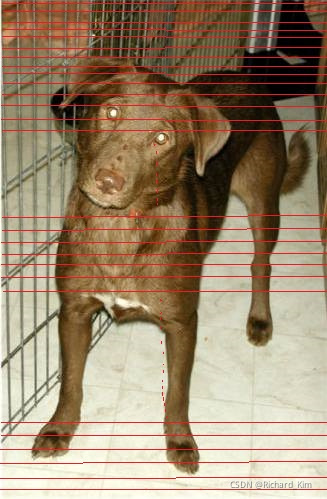
每个横向的像素作为序列。然后输入到RNN模型中。由于考虑到数据过大，所以先使用了CNN对其进行处理，CNN层会输出一个16*16*53*53的矩阵。

       RNN模型的超参数

BATCH_SIZE = 32  # 每批处理的数据 

DEVICE = torch.device('cuda' if torch.cuda.is_available() else 'cpu') 

EPOCHS = 15  # 训练数据集的轮次

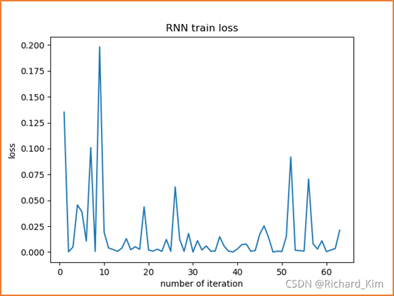
1. 最后一个epoch（第15个epoch）时候的训练集的损失率

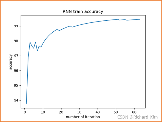
2. 最后一个epoch时候的训练准确率

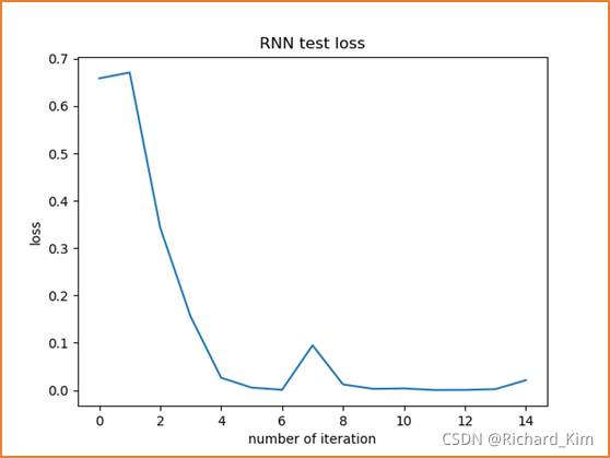
3. 总共15个epoch，每次epoch之后都测试一次，得到15次的loss

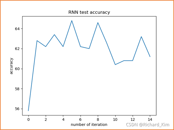
4. 每次训练完epoch之后在测试集的准确度

#!/usr/bin/env python
# -#-coding:utf-8 -*-
# author: vv
# datetime:2021/10/15  17:18:37
# software:PyCharm


"""
模型1：Pytorch RNN 实现流程
    1.图片数据处理，加载数据集
    2.使得数据集可迭代（每次读取一个Batch）
    3.创建模型类
    4.初始化模型类
    5.初始化损失类
    6.训练模型
"""

# 1.加载库
import os
import numpy as np
import torch
import torch.nn as nn
import torch.nn.functional as F
import torch.optim as optim
import torchvision
from torch.utils.data import DataLoader
from torchvision import datasets, transforms
import matplotlib.pyplot as plt

# 2.定义超参数
BATCH_SIZE = 32  # 每批处理的数据
DEVICE = torch.device('cuda' if torch.cuda.is_available() else 'cpu')  # 放在cuda或者cpu上训练
EPOCHS = 15  # 训练数据集的轮次

# 3.构建pipeline，对图像做处理
pipeline = transforms.Compose([
    # 彩色图像转灰度图像num_output_channels默认1
    # transforms.Grayscale(num_output_channels=1),
    # 分辨率重置为256
    transforms.Resize(256),
    # 对加载的图像作归一化处理， 并裁剪为[224x224x3]大小的图像(因为这图片像素不一致直接统一)
    transforms.CenterCrop(224),
    # 将图片转成tensor
    transforms.ToTensor(),
    # 正则化，模型出现过拟合现象时，降低模型复杂度
    transforms.Normalize(mean=[0.485, 0.456, 0.406], std=[0.229, 0.224, 0.225])
])

# 图片路径(训练图片和测试图片的)
base_dir_train = 'data/train'
base_dir_test = 'data/val'
# 打印一下训练图片猫狗各多少张图片
print('train dogs total images : %d' % (len(os.listdir(base_dir_train + '\\dog'))))
print('train cats total images : %d' % (len(os.listdir(base_dir_train + '\\cat'))))
print('test cats total images : %d' % (len(os.listdir(base_dir_test + '\\cat'))))
print('test dogs total images : %d' % (len(os.listdir(base_dir_test + '\\dog'))))

# 4. 加载数据集
"""
     训练集,猫是0,狗是1，ImageFolder方法自己分类的，关于ImageFolder详见: 
    https://blog.csdn.net/weixin_42147780/article/details/102683053?utm_medium=distribute.pc_relevant.none-task-blog-2%7Edefault%7ECTRLIST%7Edefault-2.no_search_link&depth_1-utm_source=distribute.pc_relevant.none-task-blog-2%7Edefault%7ECTRLIST%7Edefault-2.no_search_link
"""
train_dataset = datasets.ImageFolder(root=base_dir_train, transform=pipeline)
print("train_dataset=" + repr(train_dataset[1][0].size()))
print("train_dataset.class_to_idx=" + repr(train_dataset.class_to_idx))

# 创建训练集的可迭代对象，一个batch_size地读取数据,shuffle设为True表示随机打乱顺序读取
train_loader = DataLoader(train_dataset, batch_size=BATCH_SIZE, shuffle=True)

# 测试集
test_dataset = datasets.ImageFolder(root=base_dir_test, transform=pipeline)
# print(test_dataset)
print("test_dataset=" + repr(test_dataset[1][0].size()))
print("test_dataset.class_to_idx=" + repr(test_dataset.class_to_idx))
# 创建测试集的可迭代对象，一个batch_size地读取数据
test_loader = DataLoader(test_dataset, batch_size=BATCH_SIZE, shuffle=True)

# 获得一批测试集的数据
images, labels = next(iter(test_loader))
print("images shape", images.shape)
print("labels shape", labels.shape)


# 5.定义函数，显示一批图片
def imShow(inp, title=None):
    # tensor转成numpy,transpose转成(通道数,长,宽)
    inp = inp.numpy().transpose((1, 2, 0))
    mean = np.array([0.485, 0.456, 0.406])  # 均值
    std = np.array([0.229, 0.224, 0.225])  # 标准差
    inp = std * inp + mean
    inp = np.clip(inp, 0, 1)  # 像素值限制在0-1之间
    plt.imshow(inp)
    if title is not None:
        plt.title(title)
    plt.pause(0.001)


# 网格显示
out = torchvision.utils.make_grid(images)
imShow(out)


# 6.定义RNN网络
class RNN_Model(nn.Module):
    def __init__(self, input_dim, hidden_dim, layer_dim, output_dim):
        super(RNN_Model, self).__init__()
        # 卷积层1：输入是224*224*3 计算(224-5)/1+1=220 即通过Conv1输出的结果是220
        self.conv1 = nn.Conv2d(3, 6, 5)  # input:3 output6 kernel:5
        # 池化层：输入是220*220*6 窗口2*2  计算(220-0)/2=110 那么通过max_pooling层输出的是110*110*6
        self.pool = nn.MaxPool2d(2, 2)
        # 卷积层2， 输入是220*220*6，计算（110 - 5）/ 1 + 1 = 106，那么通过conv2输出的结果是106*106*16
        self.conv2 = nn.Conv2d(6, 16, 5)  # input:6, output:16, kernel:5
        # 以下是RNN的属性
        self.hidden_dim = hidden_dim
        self.layer_dim = layer_dim
        """
            batch_first：当 batch_first设置为True时，输入的参数顺序变为：
            x：[batch, seq_len, input_size]，
            h0：[batch, num_layers, hidden_size]。
        """
        self.rnn = nn.RNN(input_dim, hidden_dim, layer_dim, batch_first=True, nonlinearity='relu')
        # 全连接层
        self.fc1 = nn.Linear(hidden_dim, output_dim)

    def forward(self, x):
        # 卷积1
        """
        224x224x3 --> 110x110x6 -->106x106*6
        """
        x = self.pool(F.relu(self.conv1(x)))
        # 卷积2
        """
        106x106x6 --> 53x53x16 
        """
        x = self.pool(F.relu(self.conv2(x)))
        # print("x shape After CNN", x.shape)
        # x = x.reshape(x.size(0), 1, -1)  # 下面可以换成这句
        x = x.view(x.size(0), 1, -1)
        # print("x.size(0) = ", x.size(0))
        # print("x data After CNN and reshape", x.data)
        # 初始化隐藏层状态 (layer_dim,batch_size,hidden_dim),梯度运算
        h0 = torch.zeros(self.layer_dim, x.size(0), self.hidden_dim).requires_grad_().to(DEVICE)
        """
            RNN的权值并不是单一连续的，这些权值在每一次RNN被调用的时候都会被压缩，
            会很大程度上增加显存消耗。警告里也给出了解决办法，
            使用flatten_parameters()把权重存成连续的形式，可以提高内存利用率。
        """
        self.rnn.flatten_parameters()
        # print("x shape After CNN", x.shape)
        # 分类隐藏状态，避免梯度爆炸
        out, hn = self.rnn(x, h0.detach())
        # out,hn = self.rnn(x)
        # print("out size", out.shape)
        """
            输出可以是Y向量，也可以是最后一个时刻隐含层的输出hT
            如果输出是Y向量，如下图所示，那么Y向量的结构为
            out:[seq_len, batch, hidden_size].
            
            如果输出是最后一个时刻隐含层的输出h T h_Th 
            如下图所示，那么h_t:[num_layers, batch, hidden_size]，与h0结构一样
            下面的代码只要最后一层的状态ht
        """
        out = self.fc1(out[:, -1, :])  # 中间的序列长度取-1，表示取序列中的最后一个数据，这个数据长度为hidden_dim，
        # print("after fc1 out size", out.shape)  # out size torch.Size([48, 2])
        # print("hn size", hn.shape)
        return out


# 7.初始化模型
input_dim = 44944  # 输入维度(输入的节点数量)
hidden_dim = 100  # 隐藏层的维度(每个隐藏层的节点数)
layer_dim = 2  # 2层RNN(隐藏层的数量 2层)
out_dim = 2  # 输出维度
rnn_model = RNN_Model(input_dim, hidden_dim, layer_dim, out_dim)

# 8.输出模型参数信息
length = len(list(rnn_model.parameters()))
print(length)

# 9.输出模型参数信息
length = len(list(rnn_model.parameters()))
print(length)

# 优化器
# optimizer = optim.SGD(rnn_model.parameters(), lr=1e-3, momentum=0.9)
optimizer = optim.Adam(rnn_model.parameters(), lr=1e-3, betas=(0.9, 0.99))

# 损失函数,交叉熵损失函数
criterion = nn.CrossEntropyLoss()

# 把损失，准确度，迭代都记录出list，然后讲loss和准确度画出图像
sequence_dim = 53
train_loss_list = []
train_accuracy_list = []
train_iteration_list = []
test_loss_list = []
test_accuracy_list = []
test_iteration_list = []

iteration = 0
# for i, (imgs, labels) in enumerate(test_loader):
#     # print("imgs=" + repr(imgs))
#     print("labels=" + repr(labels))
#     print("i=" + repr(i))


# 训练
# """
for epoch in range(EPOCHS):
    # 用来显示训练的loss correct等
    train_correct = 0.0
    train_total = 0.0
    for i, (imgs, labels) in enumerate(train_loader):
        # 声明训练，loss等只能在train mode下进行运算
        rnn_model.train()
        # 把训练的数据集合都扔到对应的设备去
        # imgs = imgs.view(-1,1,sequence_dim, input_dim).requires_grad_().to(DEVICE)
        # print("imgs shape", imgs.shape)
        # print("imgs = ", imgs.data)
        imgs = imgs.to(DEVICE)
        labels = labels.to(DEVICE)
        # 防止梯度爆炸，梯度清零
        optimizer.zero_grad()
        # 前向传播
        rnn_model = rnn_model.cuda()  # 这里要从cuda()中取得，不然前面都放在cuda后面放在cpu，会报错，报“不在同一个设备的错误" Input and parameter tensors are not at the same device, found input tensor at cuda:0 and parameter tensor at cpu
        output = rnn_model(imgs)
        # print("RNN output shape", out.shape)
        # print("label shape", labels.shape)
        # 计算损失
        loss = criterion(output, labels)
        # 反向传播
        loss.backward()
        # 更新参数         
        optimizer.step()
        # 计算训练时候的准确度
        train_predict = torch.max(output.data, 1)[1]
        if torch.cuda.is_available():
            train_correct += (train_predict.cuda() == labels.cuda()).sum()
        else:
            train_correct += (train_predict == labels).sum()
        train_total += labels.size(0)
        accuracy = train_correct / train_total * 100.0
        # 只画出最后一次epoch的
        if (epoch + 1) == EPOCHS:
            # 迭代计数器++
            iteration += 1
            train_accuracy_list.append(accuracy)
            train_iteration_list.append(iteration)
            train_loss_list.append(loss)
        # 打印信息
        print("Epoch :%d , Batch : %5d , Loss : %.8f,train_correct:%d,train_total:%d,accuracy:%.6f" % (
            epoch + 1, i + 1, loss.item(), train_correct, train_total, accuracy))
    print("==========================预测开始===========================")
    rnn_model.eval()
    # 验证accuracy
    correct = 0.0
    total = 0.0
    # 迭代测试集 获取数据 预测
    for j, (datas, targets) in enumerate(test_loader):
        datas = datas.to(DEVICE)
        targets = targets.to(DEVICE)
        # datas = datas.view(-1, sequence_dim, input_dim).requires_grad_().to(DEVICE)
        # datas = datas.reshape(datas.size(0), 1, -1)
        # 模型预测
        outputs = rnn_model(datas)
        # 防止梯度爆炸，梯度清零
        optimizer.zero_grad()
        # 获取测试概率最大值的下标
        predicted = torch.max(outputs.data, 1)[1]
        # 统计计算测试集合
        total += targets.size(0)
        if torch.cuda.is_available():
            # print(predicted.cuda() == targets.cuda())
            correct += (predicted.cuda() == targets.cuda()).sum()
        else:
            correct += (predicted == targets).sum()
    accuracy = correct / total * 100.0
    test_accuracy_list.append(accuracy)
    test_loss_list.append(loss.item())
    test_iteration_list.append(epoch)
    print("TEST--->loop : {}, Loss : {}, correct:{}, total:{}, Accuracy : {}".format(iteration, loss.item(), correct,
                                                                                     total, accuracy))
# 可视化训练集loss
plt.figure(1)
plt.plot(train_iteration_list, train_loss_list)
plt.xlabel("number of iteration")
plt.ylabel("loss")
plt.title("RNN train loss")
plt.show()

# 可视化训练集accuracy
plt.figure(2)
plt.plot(train_iteration_list, train_accuracy_list)
plt.xlabel('number of iteration')
plt.ylabel('accuracy')
plt.title('RNN train accuracy')
plt.show()

# 可视化测试集loss
plt.figure(3)
plt.plot(test_iteration_list, test_loss_list)
plt.xlabel('number of iteration')
plt.ylabel('loss')
plt.title('RNN test loss')
plt.show()

# 可视化测试集accuracy
plt.figure(4)
plt.plot(test_iteration_list, test_accuracy_list)
plt.xlabel('number of iteration')
plt.ylabel('accuracy')
plt.title('RNN test accuracy')
plt.show()