前言
使用caffe也有一小段时间了,但是对于caffe的python接口总是一知半解,最近终于能静下心来,仔细阅读了caffe官方例程,并写下此博客。博文主要对caffe自带的分类例程00-classification.ipynb做了详细的注释,相信能加强这方面的理解。
准备工作
加载必要的库
import numpy as np
import matplotlib.pyplot as plt
%matplotlib inline
plt.rcParams['figure.figsize'] = (10, 10)
plt.rcParams['image.interpolation'] = 'nearest'
plt.rcParams['image.cmap'] = 'gray'
加载caffe
import sys
caffe_root = '../'
sys.path.insert(0, caffe_root + 'python')
import caffe
import os
if os.path.isfile(caffe_root + 'models/bvlc_reference_caffenet/bvlc_reference_caffenet.caffemodel'):
print 'CaffeNet found.'
else:
print 'Downloading pre-trained CaffeNet model...'
!../scripts/download_model_binary.py ../models/bvlc_reference_caffenet
加载网络以及输入预处理
设置cpu模式以及从硬盘加载网络
caffe.set_mode_cpu()
model_def = caffe_root + 'models/bvlc_reference_caffenet/deploy.prototxt'
model_weights = caffe_root + 'models/bvlc_reference_caffenet/bvlc_reference_caffenet.caffemodel'
net = caffe.Net(model_def,
model_weights,
caffe.TEST)
图像预处理
mu = np.load(caffe_root + 'python/caffe/imagenet/ilsvrc_2012_mean.npy')
mu = mu.mean(1).mean(1)
print 'mean-subtracted values:', zip('BGR', mu)
transformer = caffe.io.Transformer({'data': net.blobs['data'].data.shape})
transformer.set_transpose('data', (2,0,1))
transformer.set_mean('data', mu)
transformer.set_raw_scale('data', 255)
transformer.set_channel_swap('data', (2,1,0))
- 1
- 2
- 3
- 4
- 5
- 6
- 7
- 8
- 9
- 10
- 11
- 12
- 13
- 14
- 15
- 16
- 17
- 18
运行CPU分类程序
载入图片
net.blobs['data'].reshape(50,
3,
227, 227)
image = caffe.io.load_image(caffe_root + 'examples/images/cat.jpg')
transformed_image = transformer.preprocess('data', image)
plt.imshow(image)

进行分类,获取结果
net.blobs['data'].data[...] = transformed_image
output = net.forward()
output_prob = output['prob'][0]
print 'predicted class is:', output_prob.argmax()
网络输出是一个概率向量,最可能的类别是第281个类别。但是结果是否正确呢,需要查看一下ImageNet的标签。
labels_file = caffe_root + 'data/ilsvrc12/synset_words.txt'
if not os.path.exists(labels_file):
!../data/ilsvrc12/get_ilsvrc_aux.sh
labels = np.loadtxt(labels_file, str, delimiter='\t')
print 'output label:', labels[output_prob.argmax()]
打印结果如下:
output label: n02123045 tabby, tabby cat
top_inds = output_prob.argsort()[::-1][:5]
print 'probabilities and labels:'
zip(output_prob[top_inds], labels[top_inds])
打印结果如下:
probabilities and labels:
[(0.31243545, ‘n02123045 tabby, tabby cat’),
(0.23797165, ‘n02123159 tiger cat’),
(0.12387225, ‘n02124075 Egyptian cat’),
(0.10075709, ‘n02119022 red fox, Vulpes vulpes’),
(0.07095667, ‘n02127052 lynx, catamount’)]
%timeit net.forward()
1 loop, best of 3: 4.52 s per loop,结果比较慢。
gpu模式运行
caffe.set_device(0)
caffe.set_mode_gpu()
net.forward()
%timeit net.forward()
1 loop, best of 3: 196 ms per loop,简直飞起来了。
测试中间输出结果
中间层的可视化
卷积神经网络不单单是一个黑盒子。我们接下来看看该模型的一些参数和一些中间输出。首先,我们来看下如何读取网络的结构(每层的名字以及相应层的参数)。
net.blob对应网络每一层数据,对于每一层,都是四个维度:(batch_size, channel_dim, height, width)。
for layer_name, blob in net.blobs.iteritems():
print layer_name + '\t' + str(blob.data.shape)
打印结果如下:
data (50, 3, 227, 227)
conv1 (50, 96, 55, 55)
pool1 (50, 96, 27, 27)
norm1 (50, 96, 27, 27)
conv2 (50, 256, 27, 27)
pool2 (50, 256, 13, 13)
norm2 (50, 256, 13, 13)
conv3 (50, 384, 13, 13)
conv4 (50, 384, 13, 13)
conv5 (50, 256, 13, 13)
pool5 (50, 256, 6, 6)
fc6 (50, 4096)
fc7 (50, 4096)
fc8 (50, 1000)
prob (50, 1000)
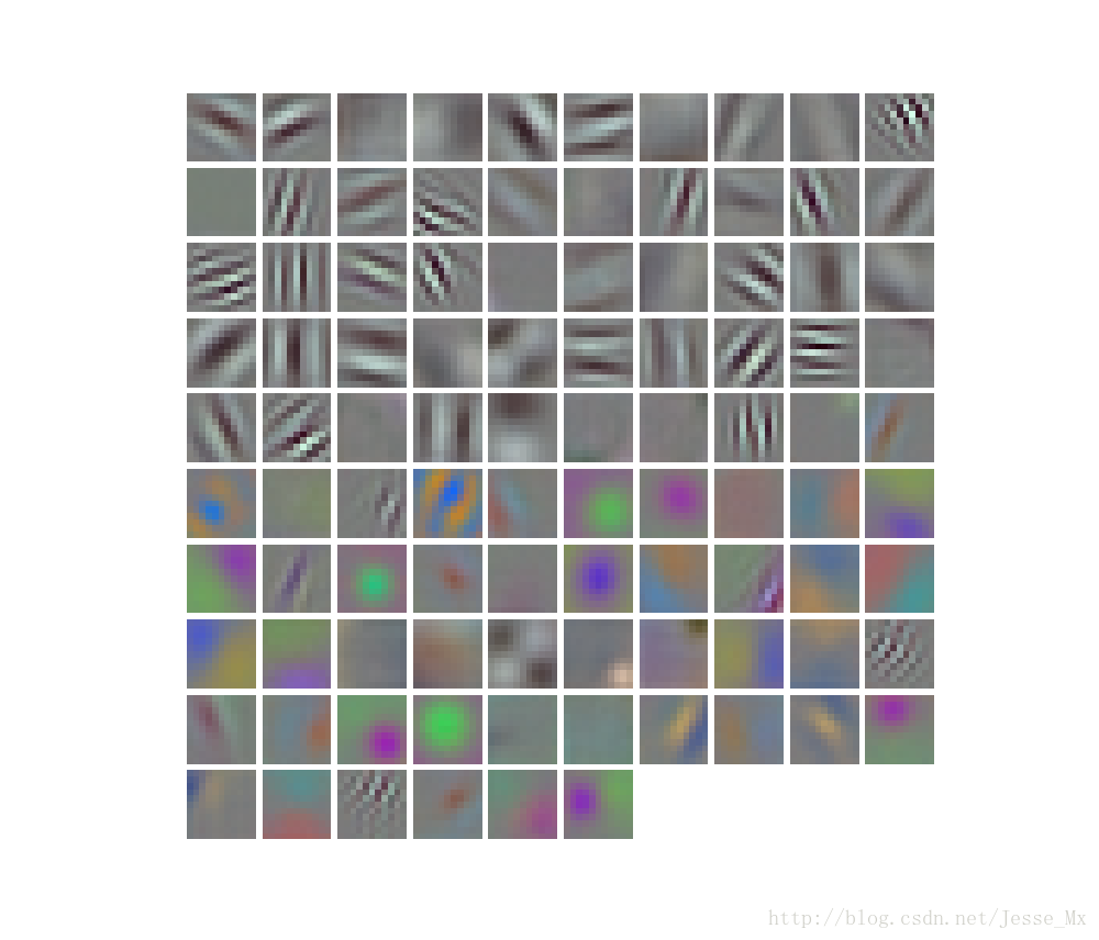
net.params对应网络中的参数(卷积核参数,全连接层参数等),有两个字典值,net.params[0]是权值(weights),net.params[1]是偏移量(biases),权值参数的维度表示是(output_channels, input_channels, filter_height, filter_width),偏移量参数的维度表示(output_channels,)
for layer_name, param in net.params.iteritems():
print layer_name + '\t' + str(param[0].data.shape), str(param[1].data.shape)
打印结果如下:
conv1 (96, 3, 11, 11) (96,)
conv2 (256, 48, 5, 5) (256,)
conv3 (384, 256, 3, 3) (384,)
conv4 (384, 192, 3, 3) (384,)
conv5 (256, 192, 3, 3) (256,)
fc6 (4096, 9216) (4096,)
fc7 (4096, 4096) (4096,)
fc8 (1000, 4096) (1000,)
这里要将四维数据进行特征可视化,需要一个定义辅助函数:
def vis_square(data):
data = (data - data.min()) / (data.max() - data.min())
n = int(np.ceil(np.sqrt(data.shape[0])))
padding = (((0, n ** 2 - data.shape[0]),
(0, 1), (0, 1))
+ ((0, 0),) * (data.ndim - 3))
data = np.pad(data, padding, mode='constant', constant_values=1) 每张小图片向周围扩展一个白色像素
data = data.reshape((n, n) + data.shape[1:]).transpose((0, 2, 1, 3) + tuple(range(4, data.ndim + 1)))
data = data.reshape((n * data.shape[1], n * data.shape[3]) + data.shape[4:])
plt.imshow(data); plt.axis('off')
- 1
- 2
- 3
- 4
- 5
- 6
- 7
- 8
- 9
- 10
- 11
- 12
- 13
- 14
- 15
- 16
- 17
- 18
- 19
- 20
- 21
- 22
- 23
filters = net.params['conv1'][0].data
vis_square(filters.transpose(0, 2, 3, 1))
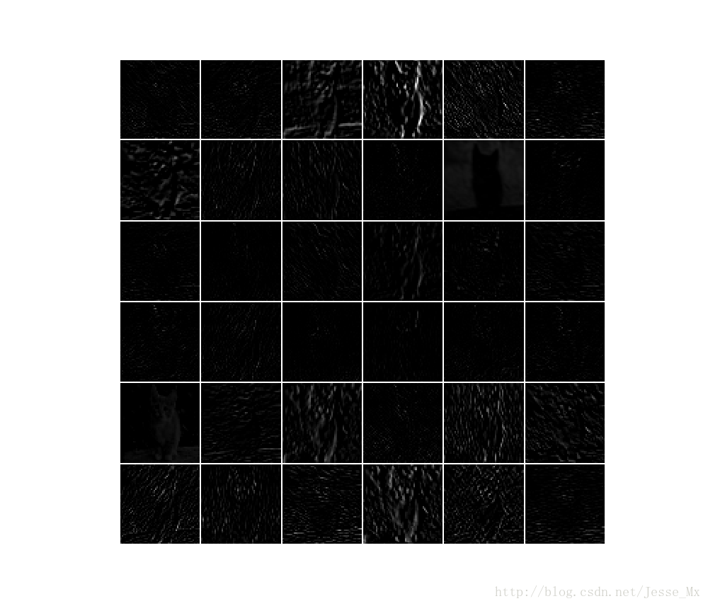
feat = net.blobs['conv1'].data[0, :36]
vis_square(feat)
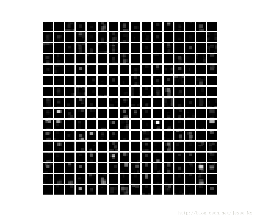
feat = net.blobs['pool5'].data[0]
vis_square(feat)
直方图显示
feat = net.blobs['fc6'].data[0]
plt.subplot(2, 1, 1)
plt.plot(feat.flat)
plt.subplot(2, 1, 2)
_ = plt.hist(feat.flat[feat.flat > 0], bins=100)
plt.show()

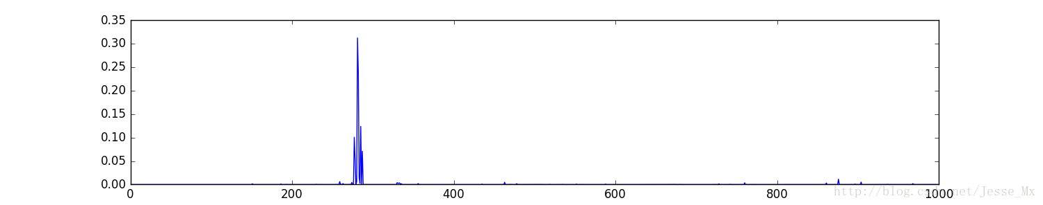
feat = net.blobs['prob'].data[0]
plt.figure(figsize=(15, 3))
plt.plot(feat.flat)
plt.show()
测试自己的图片
my_image_url = "..."
!wget -O image.jpg $my_image_url
image = caffe.io.load_image('image.jpg')
net.blobs['data'].data[...] = transformer.preprocess('data', image)
net.forward()
output_prob = net.blobs['prob'].data[0]
top_inds = output_prob.argsort()[::-1][:5]
plt.imshow(image)
plt.show()
print 'probabilities and labels:'
zip(output_prob[top_inds], labels[top_inds])
- 1
- 2
- 3
- 4
- 5
- 6
- 7
- 8
- 9
- 10
- 11
- 12
- 13
- 14
- 15
- 16
- 17
- 18
- 19
- 20
- 21
附:forward函数说明
Net_forward(self, blobs=None, start=None, end=None, **kwargs) method of caffe._caffe.Net instance
Forward pass: prepare inputs and run the net forward.
Parameters
----------
blobs : list of blobs to return in addition to output blobs.
kwargs : Keys are input blob names and values are blob ndarrays.
         For formatting inputs for Caffe, see Net.preprocess().
         If None, input is taken from data layers.
start : optional name of layer at which to begin the forward pass
end : optional name of layer at which to finish the forward pass
      (inclusive)

Returns
-------
outs : {blob name: blob ndarray} dict.


 517
517

 被折叠的 条评论
为什么被折叠?
被折叠的 条评论
为什么被折叠?
 到【灌水乐园】发言


