


英文是纯手打的!论文原文的summarizing and paraphrasing。可能会出现难以避免的拼写错误和语法错误,若有发现欢迎评论指正!文章偏向于笔记,谨慎食用!
目录
2.3.1. Multivariate distance graph construction
2.3.2. Population-wise and parcellation-wise learning
2.3.3. Parcellation-wise gradient class activation maps
2.5.1. Evaluation of disease prediction
2.5.2. Evaluation of model interpretability
2.6.1. The advantages of MDCN for brain connectome study
2.6.2. Investigation of findings
2.6.3. Limitations and future work
1. 省流版
1.1. 心得
(1)很长的Introduction!但是能直观地一开始就看到数据集和贡献
(2)可以见得作者的数学功底很好啊...公式读了半天。但是我读懂公式有什么意义呢,哎,我自己又写不出来
(3)作者常常提到xxx模型优于yyy模型因为什么什么然后又zzz模型优于nnn模型因为啥但是我压根一个都不知道啊(大脑的贫瘠
(4)⭐很出彩的一点是作者没有将重心放在精度比较上!而是考虑了两个模型的重合比较来判断疾病的同源性,感觉对医学有实质性的贡献
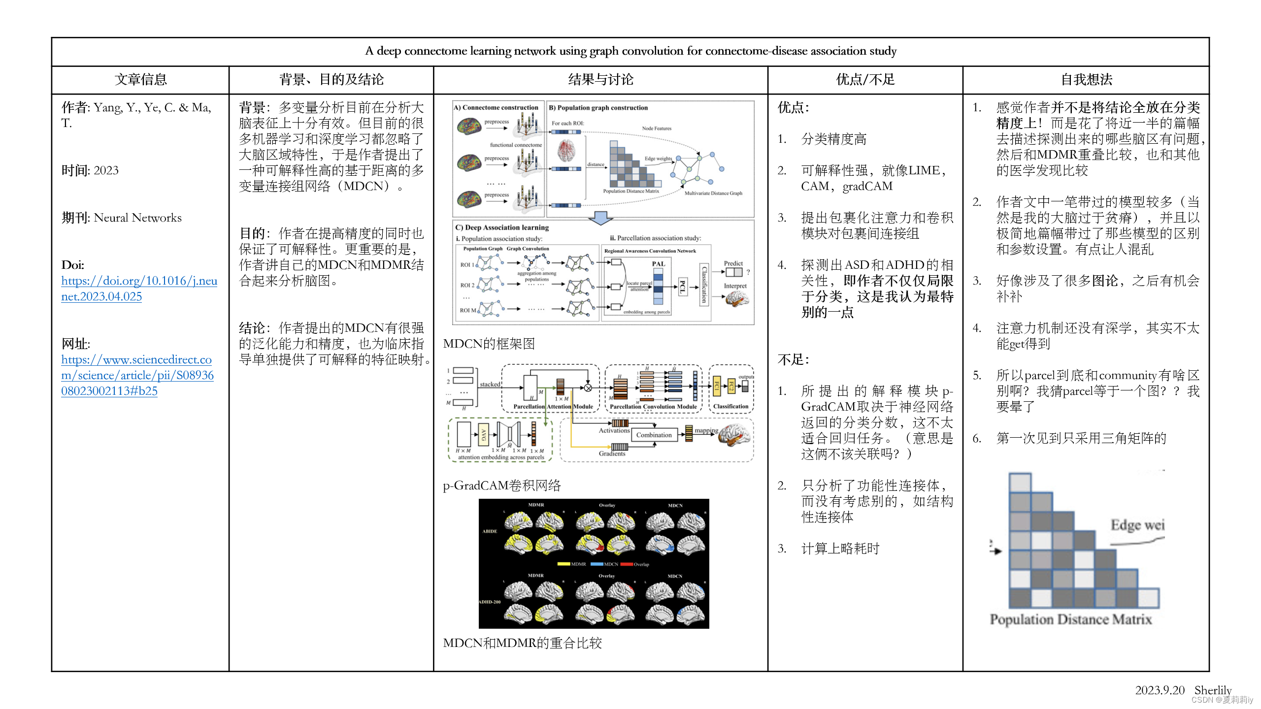
1.2. 论文框架图
2. 原文逐段精读
2.1. Abstract
Authors put forward a multivariate distance-based connectome network (MDCN) guided by connectome-wide association studies (CWAS) to solve local specificity problem and present individual differences. Then, they combine ASD, ADHD and HC to estimate the usability of their model.
phenotype adj./n.表型(的),表现型(的)(基因和环境作用的结合而形成的一组生物特征)
connectome n.连接体
2.2. Introduction
(1)Decoding neural communication, connectome, and functional activity might present the connection between individual organization and phenotypes.
(2)Neuroimaging techniques promoted the progress of medicine
(3)CWAS put all the brain networt into consider instead of separately
(4)Analytical method under CWAS framework
①Network-based statistical (NBS) analysis: avoiding multiple comparisons problems
②Multivariate distance matrix regression (MDMR) : "systematic quantification of connectome reorganization across the whole-brain network without any prior parameters"
(5)However, methods above lack of the ability of linking single variation to brain disorders
(6)Deep learning can embed features in low dimension while keeping high no-linear information
(7)Authors challenge that existing GNN models might ignore the local specificity in the brain
aberrant adj.异常的;反常的;违反常规的
2.3. Methodology
Construction shows below
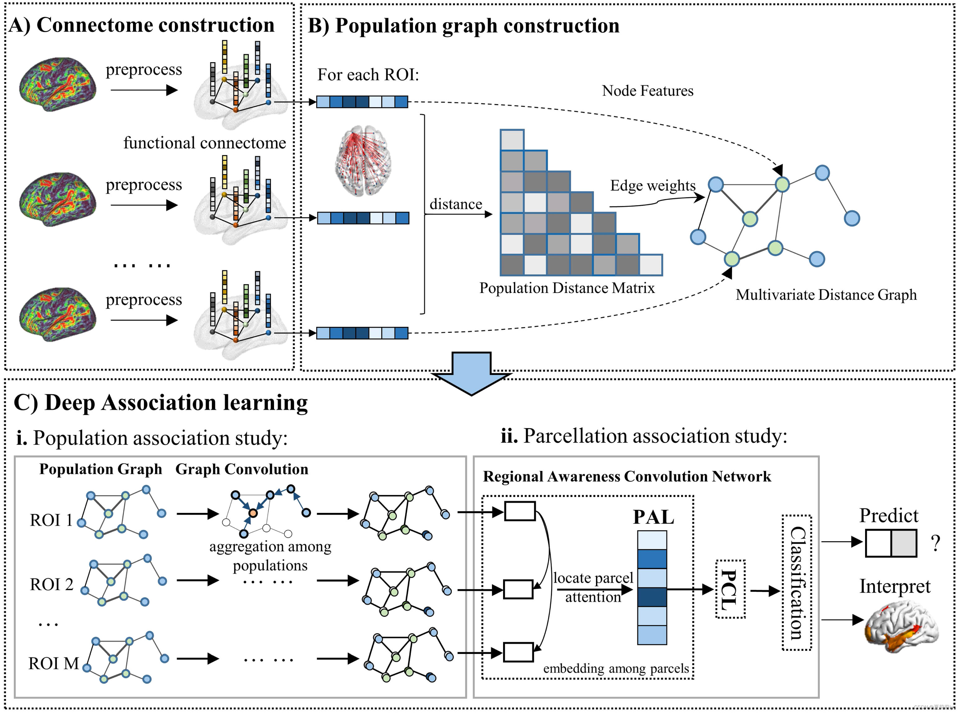
①A)They are different ROIs
②C)ii. Processing data by Parcellation-wise Attention Layer (PAL) and Parcellation-wise Convolution Layer (PCL) modules
2.3.1. Multivariate distance graph construction
(1)Distance matrix presents the difference between each subject
(2)⭐Lower triangular matrix presents for every subjecs (N), (x, y) is the whole-brain connectivity map similarity between the subject and the
subject. Obviously, lower triangular matrix is sufficient in that (x, y) meas the same with (y, x).
(3)However there are M ROIs, every matrix should be processed by M times.
①Assume , where
.
means the similarity of two nodes.
means the distance matrix above
②Then, a matrix vector is built, where every
is a lower triangular distance matrix and
.
③To calculate , regulate
, where
④σ is distance in Gaussian probability density function(看不懂)
⑤ρ is correlation distance (看不懂)
⑥F is the covariance
⑦, where
denotes the threshold for the corresponding equipment type. In this experiment, setting it to 2 for age and 1 for gender and site ID.
⑧Define regional feature vector as .
⑨Finally, combine and
to M graphs, namely
2.3.2. Population-wise and parcellation-wise learning
(1)Parcellating in M subgraphs is for solving local specificity problem. Training includes population association learning and parcellation association learning.
(2)Population association learning
①Obtain eigenvalue matrix by decomposing the Laplacian matrix with , where
is Fourier basis.
②For every node , feature is
③They use graph Fourier transform and inverse Fourier transform (猜测文中的应该是指向量的转置,这里附上图形傅里叶变换的讲解:图卷积神经网络系列:2. | 图傅里叶变换 - 知乎 (zhihu.com))
④⭐Authors put forward a convolution: , where
is kernel,
is convolution process.
⑤They define ,
,
,
which adopts K-Order Chebyshev polynomials
⑥, where
denotes identity matrix,
is the maximum eigenvalues of
,
is vector of polynomial coefficients
(3)M ROIs in each subject compose a sequence. Adopting recurrent neural network (RNN), long-short term network (LSTM), or gated recurrent unit (GRU) is deficiency in orderly capturing and global dependencies relationship.
(4)Therefore, they propose parcellation attention module (PAM) including parcellation attention module (PAM). It is able to recalibrate the feature and auto fucos on ROI.
(5)A picture that includes the p-GradCAM method:
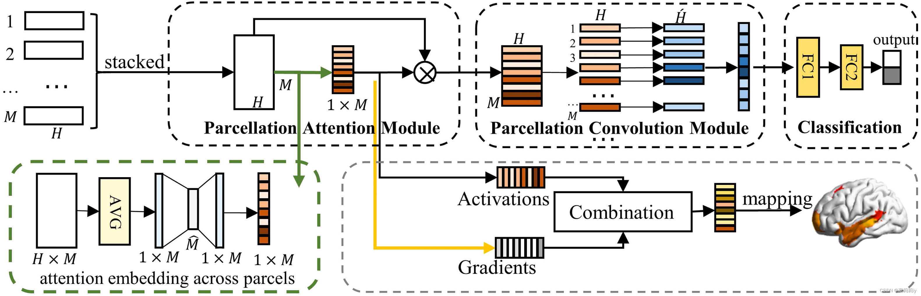
①Processing average pooling to stacked ROIs. The pool is a M*1 vector.
②Then process them by , where
and
are learnable weight(它最后又变成M*H了,文中说是什么激活重新缩放我也不知道是咋缩放啊)
③Next, in PCM layer, weighting vectors first (for every ROI, namely every row, might be different weight), then add them together to one column. (但是文中只是很vague地说权重例如聚合补丁本地信息的卷积,什么玩意儿啊)Additionally, authors use different convolution to obtain several feature map. Through this approach, more results showing.
recalibration n.重新校准;再校准;重新校正;重校
2.3.3. Parcellation-wise gradient class activation maps
(1)In this section, authors privode interpretability to their model. The activation maps designed are for locating decision region. And gradient reperesents sensitivity changes.
(2)Functions
①Similar to Grad-CAM++, authors propose the activation maps of PAM:
②Weighted average of the parcellation-wise gradients:
where denotes weighting co-efficient for the gradient,
denotes parcellation,
denotes class.
③Then
④
⑤Combining all of them, getting:
2.3.4. Optimization
(1)Authors decouple the optimization to optimization of the graph convolution network and the regional awareness convolution network.
(2)They achieve it by a two layers MLP and follows a softmax:
where and
are learnable parameters(为什么是
啊???
呢???)
(3)They choose cross-entropy function as their loss function:
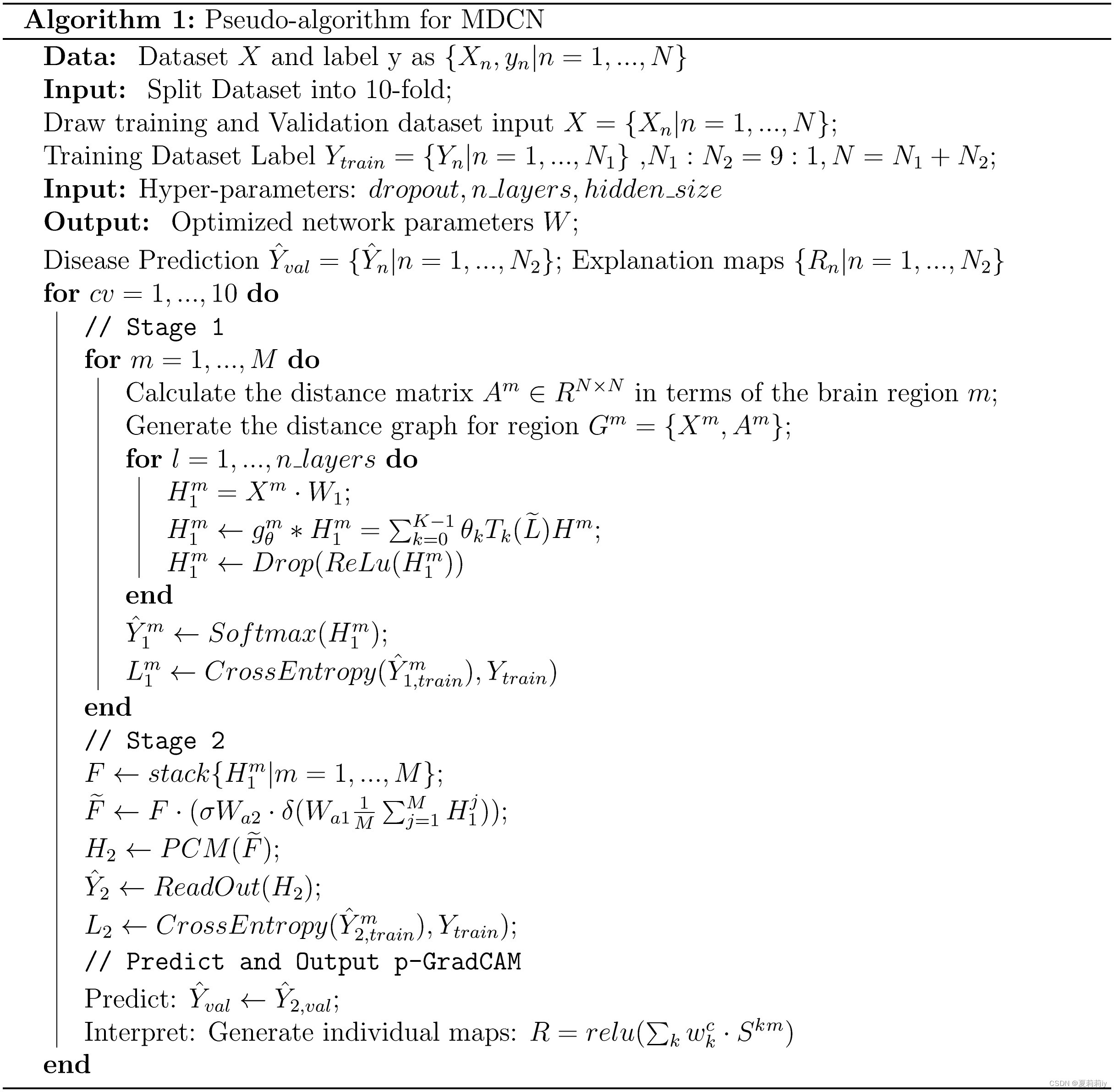
(4)Pseudo-algorithm is shown as:
decouple vt.(使两事物)分离,隔断
2.4. Experiments
2.4.1. Datasets
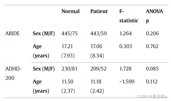
(1)They use resting-state functional MR images (fMRI) in two database to analyse
①T1 structural brain images, resting-state fMRI and phenotypic information from 17 different imaging sites in ABIDE-I database. They choose 502 ASD and 520 HC as subjects.
②They choose 261 ADHD and 311 HC ADHD-200 database
cohort n.同伙;支持者;(有共同特点或举止类同的)一群人,一批人
2.4.2. Preprocessing
(1)The ABIDE-I dataset
①Preprocess images by skull striping, slice timing correction, motion correction, global mean intensity normalization, nuisance signal regression with 24 motion parameters, and band-pass filtering (0.01–0.08 Hz). All of these are included in configurable pipeline for the analysis of connectomes (C-PAC).
②Then, register them in standard anatomical space (MNI152).
③Lastly, model nuisance variable regression with 24 motion parameters.
anatomical adj.解剖的;解剖学的;(人或动物)身体结构上的
(2)The ADHD-200 dataset
①Processing images by removing the first four volumes, slice timing correction, realignment to correct for motion, and linear transformation between the mean functional volume and the corresponding structural MRI. All of these are included in Athena pipeline incorporating AFNI and FSL neuroimaging tools.
②Then transfer images to MNI-152 space incorporating T1-weighted MRI into the MNI nonlinear warp(说实话没有很看懂这句话,我直接复制了后半句)
③Removing noise and head drifts in the time series by Nuisance regression models
④Then through band-pass filtered (0.009 Hz–0.08 Hz) denoising time series
somatomotor n.躯体运动 dorsal adj.背侧的;背部的;(鱼或动物)背上的
(3)Methods of calculating
①Mean time series for a set of regions: firstly use Schaefer template, then normalize to zero mean and unit variance
②Functional connectivity: Pearson’s Correlation Coefficient
③Regional time series: extracted by Schaefer atlas (authors adopt 100 parcels, and test 200 and 400) and then parceled by a gradient-weighted Markov random field(什么parcel过来wrap过去的)
④Each parcel matched with visual, the somatomotor, dorsal attention, salience/ventral attention, limbic, and control networks.
2.4.3. Implementations
(1)Settings
①Number of ROI: 100
②Order of Chebyshev Polynomials: 3
③GCN parameters, hidden size, number of layers: using grid search to optimize
④Drop rate: 0.3
⑤Learning rate: 0.005
⑥Weight decay for regularization: 0.0005
(2)Evaluations
①Validation: 10-fold stratified cross-validation
②Methods: prediction accuracy (ACC), sensitivity (SEN), specificity (SPE), F1 score (F1), and area under the curve (AUC)
③“在第一阶段,当验证损失达到 500 个 epoch 中的最低值时,将获得第二阶段训练的表示。第二阶段拟合训练数据集和验证数据集的嵌入式特征,并在 500 个 epoch 中进行训练。”(啥意思??先训练500个epoch然后找最小的那个loss?)
2.4.4. Competitive methods
(1)SVM: flatten triangular matrix to vector
(2)NBS/MDMR-SVM: they filter a lot of features in fuctional connectivity. Authors use grid search with range of 0.05 - 0.15 and steps of 0.005 to determine parameters. Then choose significant value which p <0.05
(3)GCN: they use semi-supervised GCN, and select feature through recursive feature elimination (RFE)
(4)BrainNetCNN: using edge-to-edge (E2E) layer with 32 channel size, edge-to-node (E2N) with 64 output features, and node-to-graph (N2G) layer with 30 output features.Then, setting drop rate as 0.5
(5)BrainGNN: setting
(6)Hypergraph Neural Network (HGNN)/Dynamic Hypergraph Neural Network (DHGNN)
(7)Hierarchical GCN (HI-GCN)/Ensemble of Transfer Hierarchical Graph Convolutional Networks (TE-HI-GCN): including hierarchical structure to show ropology information
recursive adj.递归的;循环的
2.5. Results
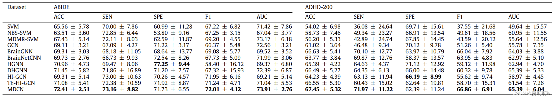
2.5.1. Evaluation of disease prediction
(1)我实在是看不懂那些方法之间的比较主要是我连那些方法都不知道是啥样的啊
(2)Classification model in two datasets
2.5.2. Evaluation of model interpretability
(1)Individual maps derived from p-GradCAM
(2)Group analysis
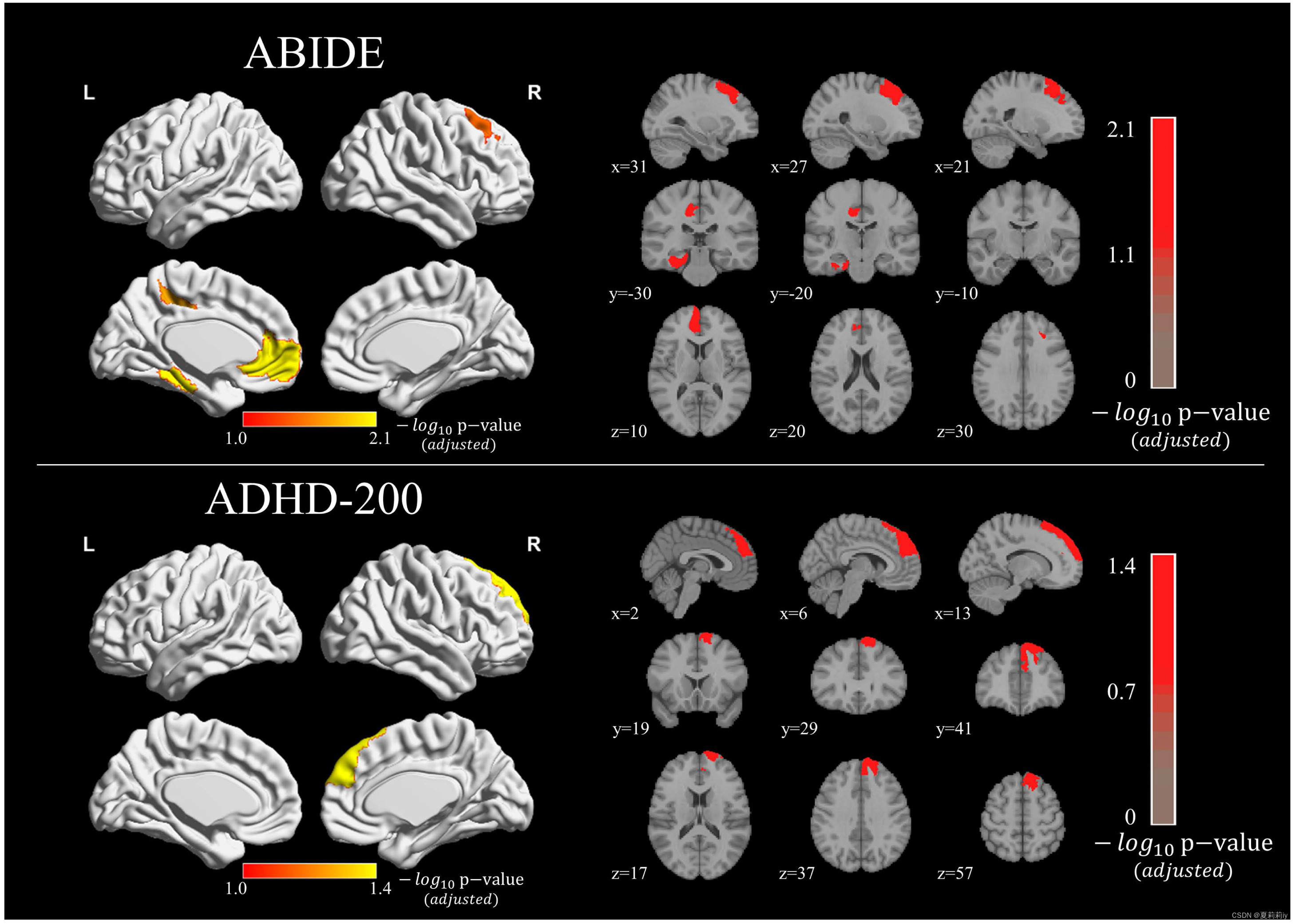
①The picture below shows the gradient and class activation maps for each dataset
②Red area denotes the amplitude of the map values. The saturation of red from light to deep denotes connection from weak to strong
③HC mostly has higher values in the medial and dorsal prefrontal cortex regions than ASD
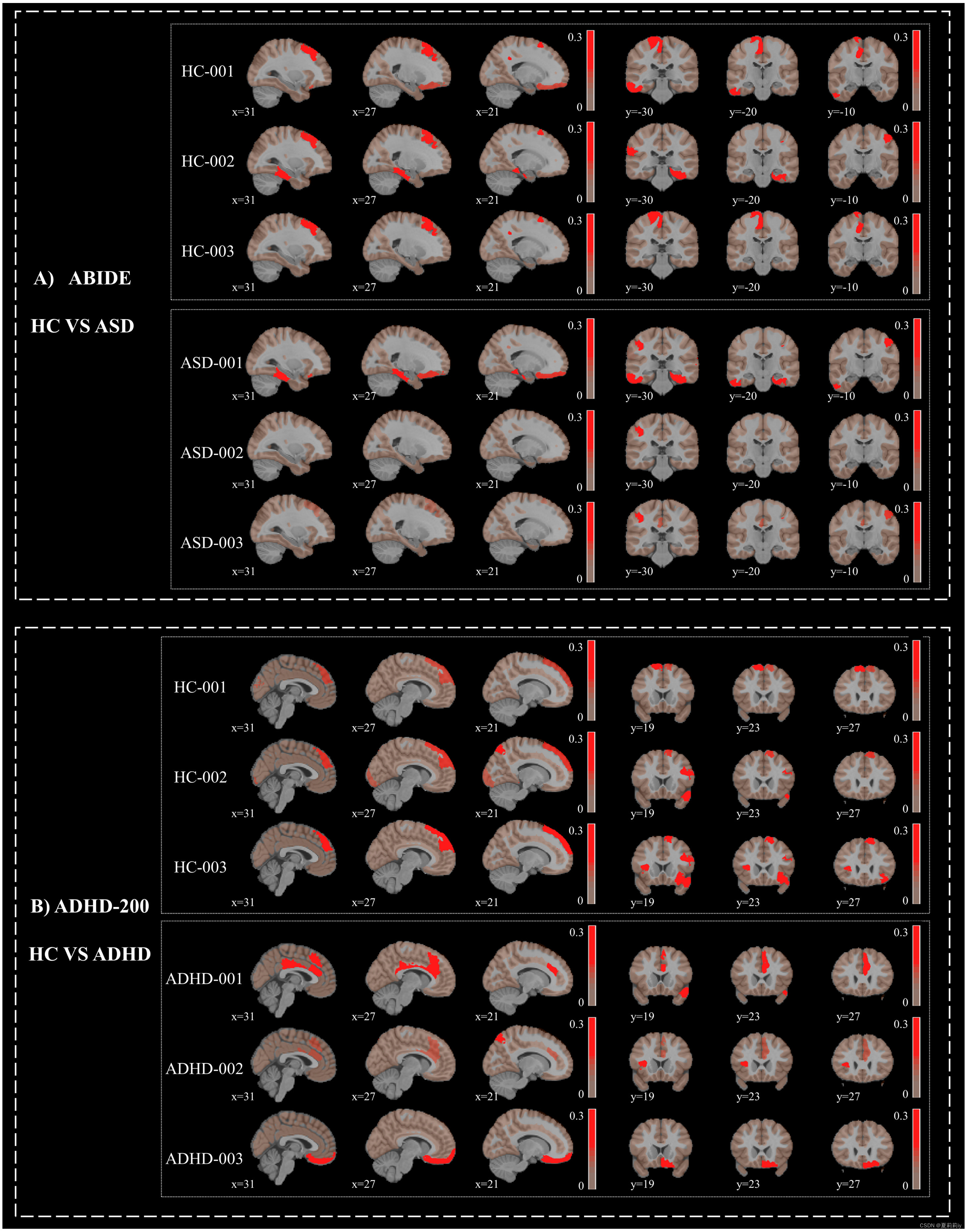
④Adopt t-test for group and control it by Bonferroni correction
⑤All these regions in datasets belong to default mode, limbic, and control networks three functional subnetworks. Default mode is found significant difference in ADHD-200, where their connectivity patterns prominently decrese
⑥The left of this picture is of axial panel, and right is of coronal panel
⑦Significant patterns (p<0.05) respectively on ABIDE and ADHD-200 show below (pictures in the right side are from axial, coronal, and sagittal panels):
(3)Comparison of MDCN findings with MDMR
①Population distance is what MDCN to measure inter- and intra-group similarities, which constructs its incredible feature
②Picture below presents MDMR, overlay, MDCN in two datasets:
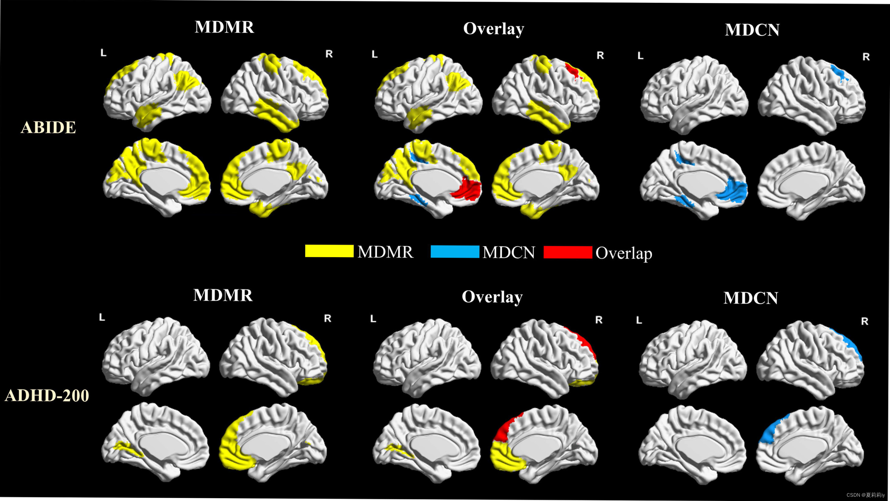
These overlayed regions are reckoned feasibility of the MDCN model (但是我觉得在ABIDE里面重合区域不多啊...)
2.5.3. Sensitivity analysis
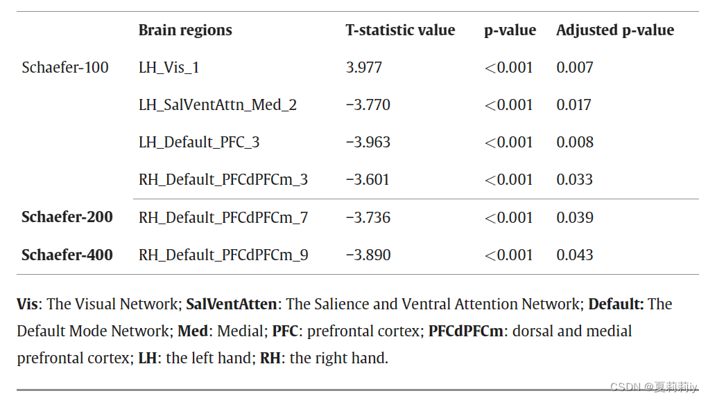
(1)State how to tune parameters in Schaefer atlas
(2)Classification accuracy reaches the highest in Schaefer-400 atlas, whereas AUC gets the best in Schaefer-100 atlas. Accordingly, authors acknowledge the generalization ability of Schaefer-100
(3)The statistical diagram of distance measurement, including the Euclidean, Chebyshev, and cosine similarity distances, is shown below:
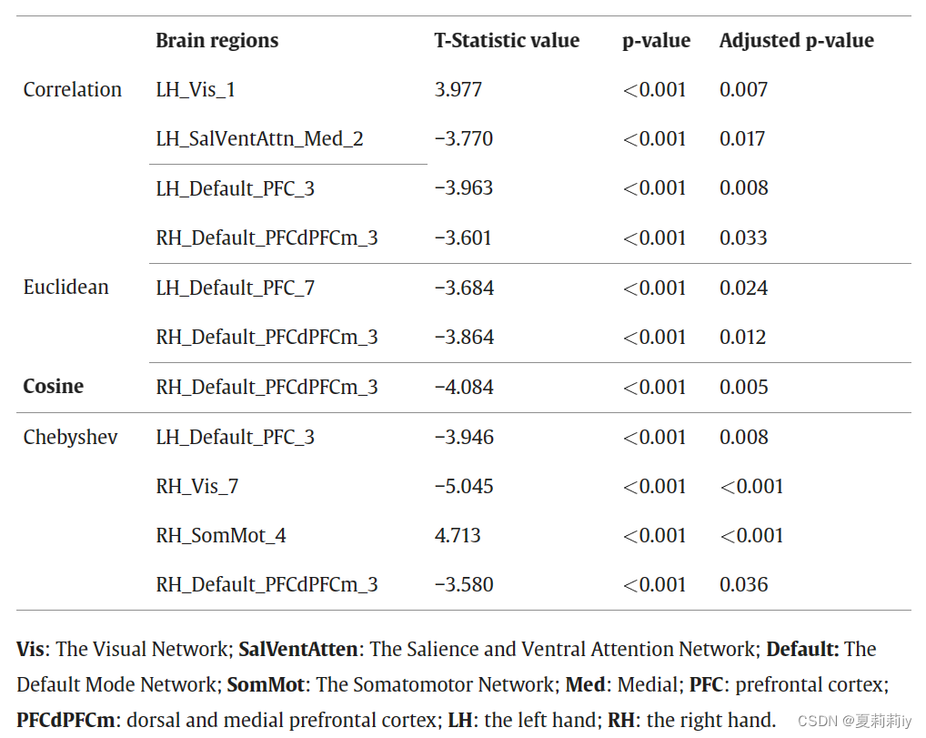
Among them, there are significant difference in the correlation and Chebyshev distance in the left prefrontal cortex
(4)Comparison pictures of three approaches
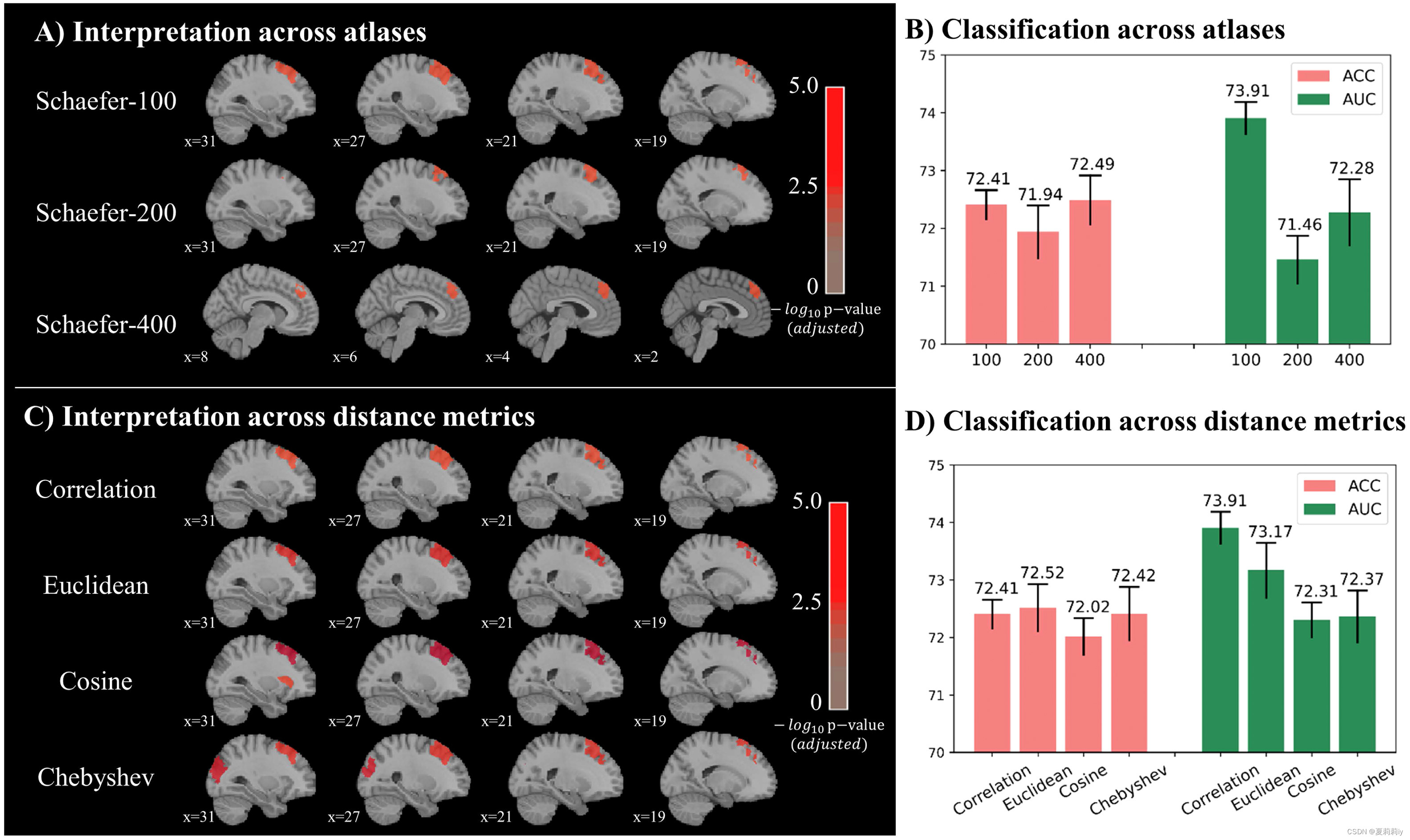
①Depth of red denotes significance
2.6. Discussion
(1)MDCN is able to transfer high-order nonlinear message between populations and parcellations. By this, it maps individual brain network signatures
(2)Authors acknowledge it's overlap region, which combine two classification methods
2.6.1. The advantages of MDCN for brain connectome study
(1)Innovations of MDCN
①GCN for population association studies
②PAM and PCM
③Interpretable p-GradCAM model
(2)Population graph: built based on features in each parcellation
(3)MDCN increases 2.41% accuracy
(4)They think there are inside problem of ABBED dataset
(5)CAM and GradCAM based on gradient are able to interpret the identification of diseases
surrogate v./n./adj.代理(的),替代(的)
ad-hoc 特别的;自组织;自组网;点对点;对等模式;
2.6.2. Investigation of findings
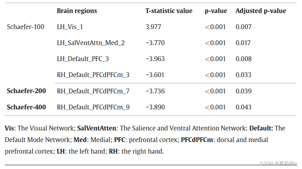
(1)Findings: for ASD, disease-specific brain functional network disturbances mostly present in left visual network, the left salience/ventral attention network and the bilateral default mode network. For ADHD, the most vulnerable region is the right default mode network.
2.6.3. Limitations and future work
(1)p-GradCAM depends on classification score returned from the neural network. Therefore, it is not suitable for regression.(我不知道为什么欸)
(2)Besides evaluating functional connectome, MDCN is expected for other classification
(3)MDCN is a little bit expensive
2.7. Conclusion
Interpretability and accuracy of MDCN are excellent
3. 概念补充
3.1. Matrix vector
(1)Concept: matrix vector space is a linear space with a matrix as its element
(2)Example: , where every
is a lower triangular distance matrix
3.2. Laplacian matrix
(1)Function:
(2)Example graph
(3) denotes matrix of degree of one node,
matrix shows as:
(4) denotes the adjacency matrix,
is as follows:
(5)Then is:
3.3. Fourier basis
(1)variations in Fourier Series in one cycle
are pairwise orthogonality. Thus, they are natural orthogonal basis
4. Reference List
Yang, Y., Ye, C. & Ma, T. (2023) 'A deep connectome learning network using graph convolution for connectome-disease association study', Neural Networks, vol. 164, pp. 91-104. doi: Redirecting


 被折叠的 条评论
为什么被折叠?
被折叠的 条评论
为什么被折叠?
 到【灌水乐园】发言


