


任务描述:临床特征 和 影像组学特征 保存在 excel 文件中,需要进行 特征筛选,然后再将筛选出来的特征利用逻辑回归进行二分类。
有如下几个问题和需求:
1. excel 中的特征都是以 str 的形式写入表格中的,读取的时候要转换成数字形式;特征之间的尺度不一样,读取出来之后需要按列进行归一化;
2. excel 中保存的标签为符号格式:IA, MIA, AAH, AIS,本任务想进行 IA vs non-IA 的二分类,需要进行标签读取和 0-1 赋值;
3. 因为要进行分类,需要划分训练集和测试集,注意⚠️,特征筛选需要在训练集上进行,训练集需要保证全流程的独立;
4. 划分训练集和测试集之后,希望将临床特征和影像组学特征分别保存,以用来比较分类性能;
5. 因为要和另一个处理流程的结果做比较,所以希望将划分的训练集和测试集保存下来,特征,对应的标签,写入 csv;
6. 利用 LASSO CV 进行特征筛选,希望实现如下几个功能:
1)阈值设定上:设置大于 0 和 大于 非零值中值 两种模式
2)将筛选出来的特征打印出来
3)将筛选出来的特征在 lasso cv 模型中的系数按照大小绘制横向柱状图
4)对筛选出来的特征进行相关性分析,绘制相关性热力图矩阵
5)只用训练集进行特征筛选,但是要从测试集中提取出来筛选的特征
7. 使用逻辑回归进行二分类,交叉验证进行模型系数优化,针对训练集和测试集分别绘制 roc 曲线,并绘制 混淆矩阵 的热力图。
代码如下:
import os
import csv
import xlrd
import numpy as np
import pandas as pd
import seaborn as sb
from sklearn import metrics
from sklearn.metrics import auc
import matplotlib.pyplot as plt
from sklearn.linear_model import LassoCV
from sklearn.metrics import confusion_matrix
from sklearn.model_selection import train_test_split
from sklearn.feature_selection import SelectFromModel
from sklearn.linear_model import LogisticRegressionCV
def MaxMinNormalization(x, Max, Min):
x = (x - Min) / (Max - Min)
return x
def lasso_selector(Xtrain, ytrain, Xtest, featuresname):
clf_fs = LassoCV(max_iter=1000).fit(Xtrain, ytrain)
importance = np.abs(clf_fs.coef_)
print(clf_fs.coef_)
threshold = 1e-16
# threshold = np.median(importance[np.nonzero(importance)])
idx_features = importance >= threshold
name_features = np.array(featuresname)[idx_features]
print('Selected features: {}'.format(name_features))
sfm = SelectFromModel(clf_fs, threshold=threshold)
sfm.fit(Xtrain, ytrain)
selected_features_train = sfm.transform(Xtrain)
selected_features_test = sfm.transform(Xtest)
# coefficients in the Lasso Model
importance_features = np.array(importance)[idx_features]
sorted_importance, sorted_name = zip(*sorted(zip(importance_features, name_features)))
plt.figure(figsize=(10, 5))
plt.barh(width=sorted_importance, y=sorted_name)
plt.title("Coefficients in the Lasso Model")
plt.tight_layout()
plt.show()
# correlation heatmap
plt.figure(figsize=(11, 10))
zipped_data = dict(zip(name_features, selected_features_train))
dataframe = pd.DataFrame(zipped_data, columns=name_features)
matrix = dataframe.corr()
sb.heatmap(matrix, cmap="RdBu")
plt.tight_layout()
plt.show()
return selected_features_train, selected_features_test
def confusion_matrix_plot(confusion_matrix):
# plt.figure()
sb.set()
f, ax = plt.subplots()
print(confusion_matrix)
sb.heatmap(confusion_matrix, annot=True, ax=ax, fmt='g')
ax.set_title('confusion matrix')
ax.set_xlabel('predict')
ax.set_ylabel('true')
plt.show()
def logisticRegressionROC(x_train, y_train, x_test, y_test):
clf_cl = LogisticRegressionCV(cv=10, random_state=1).fit(x_train, y_train)
predicted_prob_train = clf_cl.predict_proba(x_train)[:, 1]
predicted_prob_test = clf_cl.predict_proba(x_test)[:, 1]
fpr_train, tpr_train, thresholds_train = metrics.roc_curve(y_train, predicted_prob_train)
fpr_test, tpr_test, thresholds_test = metrics.roc_curve(y_test, predicted_prob_test)
roc_auc_train = auc(fpr_train, tpr_train)
roc_auc_test = auc(fpr_test, tpr_test)
predicted_train = clf_cl.predict(x_train)
predicted_test = clf_cl.predict(x_test)
confusion_matrix_plot(confusion_matrix(y_train, predicted_train, labels=[0, 1]))
confusion_matrix_plot(confusion_matrix(y_test, predicted_test, labels=[0, 1]))
return fpr_train, tpr_train, roc_auc_train, fpr_test, tpr_test, roc_auc_test
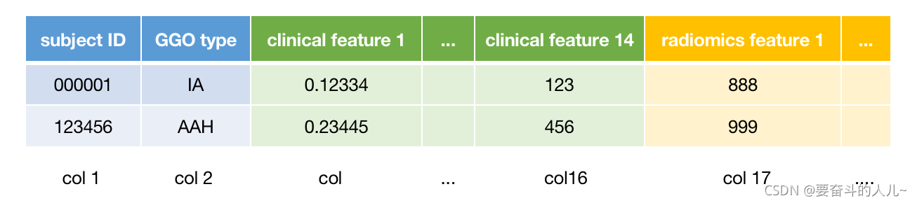
# radiomics features saved in the xlsx file
# col1: subject ID
# col2: clinical label(GGO_subtype): 'IA' 'MIA' 'AAH' 'AIS'
# col3-16: clinical features
# col17-end: radiomics features
data_path = '/data_files/临床信息+影像组学.xlsx'
dataset = xlrd.open_workbook(data_path).sheets()[0]
GGO_subtype = np.array(dataset.col_values(1))[1:]
features_name = np.array(dataset.row_values(0))[2:]
radiomics_features_name = np.array(dataset.row_values(0))[16:]
clinical_features_name = np.array(dataset.row_values(0))[2:16]
features_matrix = []
header = np.array(dataset.row_values(0))
for i in range(2, len(header)):
temp = list(map(float, np.array(dataset.col_values(i))[1:]))
features_matrix.append(MaxMinNormalization(temp, np.max(temp), np.min(temp)))
features_matrix = np.transpose(features_matrix)
two_class_label = [] # IA VS non-IA
for i in GGO_subtype:
if i == 'IA':
two_class_label.append(1)
else:
two_class_label.append(0)
# split the train and the test
X_train, X_test, y_train, y_test = train_test_split(features_matrix, two_class_label,
stratify=two_class_label, test_size=0.2, random_state=0)
X_train_radiomics, X_test_radiomics = X_train[:, 14:], X_test[:, 14:]
X_train_clinical, X_test_clinical = X_train[:, 0:14], X_test[:, 0:14]
# ########################## if you want to save the train and test set(start) ###################################### #
counter = 0
for i in range(len(X_train_radiomics)):
with open(os.path.join('/Users/Desktop/data_files', 'radiomics_train.csv'), 'a', newline='') as outcsv:
writer = csv.writer(outcsv)
if counter == 0:
writer.writerow(['patient_id', 'label'] + list(radiomics_features_name))
counter += 1
writer.writerow([str(counter), y_train[i]] + list(X_train_radiomics[i]))
counter_test = counter
for i in range(len(X_test_radiomics)):
with open(os.path.join('/Users/Desktop/data_files', 'radiomics_test.csv'), 'a', newline='') as outcsv:
writer = csv.writer(outcsv)
if counter_test == counter:
writer.writerow(['patient_id', 'label'] + list(radiomics_features_name))
counter_test += 1
writer.writerow([str(counter_test), y_test[i]] + list(X_test_radiomics[i]))
counter = 0
for i in range(len(X_train_clinical)):
with open(os.path.join('/Users/Desktop/data_files', 'clinical_train.csv'), 'a', newline='') as outcsv:
writer = csv.writer(outcsv)
if counter == 0:
writer.writerow(['patient_id', 'label'] + list(clinical_features_name))
counter += 1
writer.writerow([str(counter), y_train[i]] + list(X_train_clinical[i]))
counter_test = counter
for i in range(len(X_test_clinical)):
with open(os.path.join('/Users/Desktop/data_files', 'clinical_test.csv'), 'a', newline='') as outcsv:
writer = csv.writer(outcsv)
if counter_test == counter:
writer.writerow(['patient_id', 'label'] + list(clinical_features_name))
counter_test += 1
writer.writerow([str(counter_test), y_test[i]] + list(X_test_clinical[i]))
# ######################### if you want to save the train and test set(end) ####################################### #
# ############################################# feature selection(start) ############################################ #
selected_radiomics_features_train, selected_radiomics_features_test = lasso_selector(X_train_radiomics, y_train,
X_test_radiomics,
radiomics_features_name)
selected_clinical_features_train, selected_clinical_features_test = lasso_selector(X_train_clinical, y_train,
X_test_clinical,
clinical_features_name)
selected_all_features_train = np.concatenate((selected_radiomics_features_train, selected_clinical_features_train),
axis=1)
selected_all_features_test = np.concatenate((selected_radiomics_features_test, selected_clinical_features_test), axis=1)
# ############################################# feature selection(end) ############################################ #
# ############################################ logistic regression (start) ########################################### #
fpr_train_radiomics, tpr_train_radiomics, roc_auc_train_radiomics, fpr_test_radiomics, tpr_test_radiomics, roc_auc_test_radiomics = \
logisticRegressionROC(selected_radiomics_features_train, y_train, selected_radiomics_features_test, y_test)
fpr_train_clinical, tpr_train_clinical, roc_auc_train_clinical, fpr_test_clinical, tpr_test_clinical, roc_auc_test_clinical = \
logisticRegressionROC(selected_clinical_features_train, y_train, selected_clinical_features_test, y_test)
fpr_train_all, tpr_train_all, roc_auc_train_all, fpr_test_all, tpr_test_all, roc_auc_test_all = \
logisticRegressionROC(selected_all_features_train, y_train, selected_all_features_test, y_test)
plt.figure()
plt.plot(fpr_train_clinical, tpr_train_clinical, color="blue", lw=2)
plt.plot(fpr_train_radiomics, tpr_train_radiomics, color="darkorange", lw=2)
plt.plot(fpr_train_all, tpr_train_all, color='red', lw=2)
plt.xlabel("False Positive Rate")
plt.ylabel("True Positive Rate")
plt.title("ROC for Train")
plt.legend(['Clinical, AUC = %0.2f' % roc_auc_train_clinical, 'Radiomics, AUC = %0.2f' % roc_auc_train_radiomics,
'Clinical+Radiomics, AUC = %0.2f' % roc_auc_train_all])
plt.show()
plt.figure()
plt.plot(fpr_test_clinical, tpr_test_clinical, color="blue", lw=2)
plt.plot(fpr_test_radiomics, tpr_test_radiomics, color="darkorange", lw=2)
plt.plot(fpr_test_all, tpr_test_all, color='red', lw=2)
plt.xlabel("False Positive Rate")
plt.ylabel("True Positive Rate")
plt.title("ROC for Test")
plt.legend(['Clinical, AUC = %0.2f' % roc_auc_test_clinical, 'Radiomics, AUC = %0.2f' % roc_auc_test_radiomics,
'Clinical+Radiomics, AUC = %0.2f' % roc_auc_test_all])
plt.show()
# ############################################ logistic regression (end) ######################################### #


 1069
1069


 被折叠的 条评论
为什么被折叠?
被折叠的 条评论
为什么被折叠?
 到【灌水乐园】发言


