Dubins路径的计算和Python&Julia实现

w# DubinsPath

简介

Dubins曲线是在满足曲率约束和规定的始端和末端的切线的条件下，连接两个二维平面的最短路径，限制目标只能向前行进。

Dubins曲线的目的是规划一条满足转弯半径、前进方向、初始相对位置和速度方向的最短曲线。

Dubins曲线分类

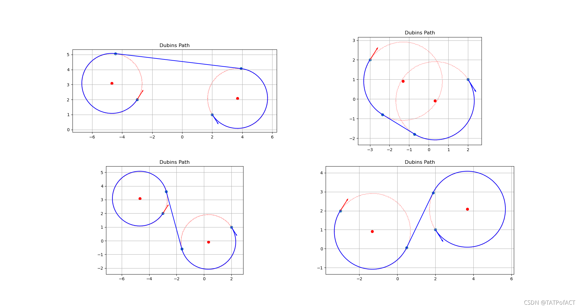
在运动方向已知和转向半径最小的情况下，从初始向量到终止向量的最短的路径是由直线和最小半径转向圆弧组成的。

• L：逆时针圆弧运动
• R：顺时针圆弧运动
• S：直线运动

计算

• 输入参数

  出发点$P_i:(x_1,y_1,\alpha )$

  终止点$P_f:(x_2,y_2,\beta )$

  转弯半径$r$

• 输出

  Dubins路径的长度和路径点

1. 坐标系转换

   将$P_i$变为新坐标系的原点，旋转坐标系使$P_f$在$X$轴上。

   $P_i:(x_1,y_1,\alpha )->P_i^{\prime }:(0,0,\alpha -\theta ({\alpha }^{\prime }))$

   $P_f:(x_2,y_2,\beta )->P_f^{\prime }:(d,0,\beta -\theta ({\beta }^{\prime }))$
   其中：
   $$\{\begin{array}{l}\theta =\arctan [(y_2-y_1)/(x_2-x_1)]\\ |\overrightarrow{P_i{P}_f}|=\sqrt{(x_1-x_2{)}^2+(y_1-y_2{)}^2}\\ d=|\overrightarrow{P_i{P}_f}|/r\end{array}$$

   转弯半径被归一化为1，可以直接使用弧度来表示路径长度。

2. 计算Dubins路径长度

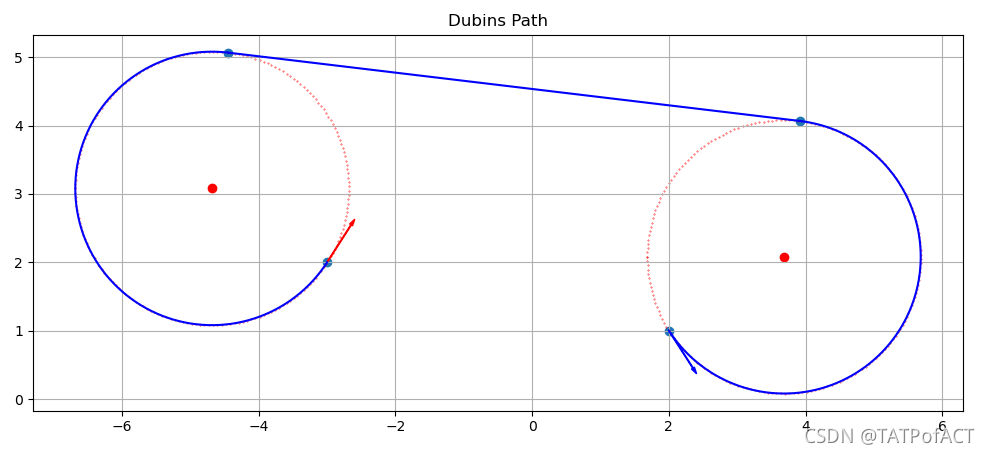
• RSR型路径

  1. 根据起始点的坐标和方向推算出圆心的坐标
  2. 找到两圆的公切线中满足逆时针方向的那一条

• LSL型路径

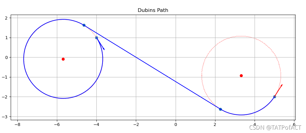
• LSR型路径

3. 坐标系转换

python代码实现

文字部分后续补全，代码如下：

import numpy as np
import matplotlib.pyplot as plt
from math import pi, sin, cos, acos, atan2, sqrt

##########################################################
# 功能:
#   输入起止点的坐标,方向,转弯半径,曲线的种类，计算Dubins曲线
#
# 输入参数:
#   起点坐标:
#       Pi(x,y)
#   终点坐标:
#       Pf(x,y)
#   起点角度:
#       alpha(弧度)
#   终点角度:
#       beta(弧度)
#   转弯半径:
#       ratio
#   曲线类型:
#       tp "RSR","LSL","RSL","LSR"
#       ( R顺时针 L逆时针 S直线 default："RSR" )
#   是否可视化结果:
#       show_path (default=True)
#
# 输出结果：三元组
#   切出点坐标posiA:[A_x,A_y]
#   切入点坐标posiB:[B_x,B_y]
#   三段距离dist lst:[dist1出发圆弧,dist2直线,dist3到达圆弧
#
# Author: jia-yf19@mails.tsinghua.edu.cn
# Date  : 2021.10.28
#
##########################################################
def Dubins_path(Pi, Pf, alpha, beta, ratio, tp="RSR", show_path=True):
    assert len(Pi) == 2 and len(Pf) == 2
    assert tp in ["RSR", "LSL", "RSL", "LSR"]
    assert ratio > 0.

    # 坐标变换
    Vec_Move = np.matrix([[1., 0., -Pi[0]], [0., 1., -Pi[1]], [0., 0., 1.]])  # 平移
    temp_theta = -(atan2(Pf[1] - Pi[1], Pf[0] - Pi[0]) + pi)
    alpha_ = alpha + temp_theta
    beta_ = beta + temp_theta
    Vec_Rotate = np.matrix([[cos(temp_theta), -sin(temp_theta), 0.],
                            [sin(temp_theta), cos(temp_theta), 0.], 
                            [0., 0., 1.]])  # 旋转
    Vec_Length = np.matrix([[1. / ratio, 0., 0.],
                            [0., 1. / ratio, 0.],
                            [0., 0., 1.]])  # 拉伸
    Vec_Trans = Vec_Length * Vec_Rotate * Vec_Move  # 变换矩阵

    temp_res = Vec_Trans * [[Pi[0]], [Pi[1]], [1]]
    Pi_ = [temp_res[0, 0], temp_res[1, 0]]
    temp_res = Vec_Trans * [[Pf[0]], [Pf[1]], [1]]
    Pf_ = [temp_res[0, 0], temp_res[1, 0]]

    # 曲线计算
    if tp == "RSR":  # 双逆时针路线
        O1_x, O1_y = sin(alpha_), -cos(alpha_)          # 起点圆
        O2_x, O2_y = Pf_[0] + sin(beta_), -cos(beta_)   # 终点圆
        theta = atan2(O2_y - O1_y, O2_x - O1_x)         # 圆心夹角
        pho1 = (theta - alpha_) % (2.0 * pi)            # 起点圆弧度
        pho2 = sqrt((O1_x - O2_x)**2 + (O1_y - O2_y)**2)    # 直线长度
        pho3 = (beta_ - pho1 - pho2 - alpha_) % (2.0 * pi)  # 终点圆弧度
        A_x, A_y = sin(alpha_) - sin(alpha_ + pho1), -cos(alpha_) + cos(alpha_ + pho1)          # 切出点
        B_x, B_y = Pf_[0] + sin(beta_) - sin(alpha_ + pho1), -cos(beta_) + cos(alpha_ + pho1)   # 切入点
    elif tp == "LSL":  # 双顺时针路线
        O1_x, O1_y = -sin(alpha_), cos(alpha_)          # 起点圆
        O2_x, O2_y = Pf_[0] - sin(beta_), cos(beta_)    # 终点圆
        theta = atan2(O2_y - O1_y, O2_x - O1_x)         # 圆心夹角
        pho1 = (theta - alpha_) % (2.0 * pi)            # 起点圆弧度
        pho2 = sqrt((O1_x - O2_x)**2 + (O1_y - O2_y)**2)    # 直线长度
        pho3 = (beta_ - pho1 - pho2 - alpha_) % (2.0 * pi)  # 终点圆弧度
        A_x, A_y = -sin(alpha_) + sin(alpha_ + pho1), cos(alpha_) - cos(alpha_ + pho1)          # 切出点
        B_x, B_y = Pf_[0] - sin(beta_) + sin(alpha_ + pho1), cos(beta_) - cos(alpha_ + pho1)    # 切入点
    elif tp == "RSL":  # 八字交叉路线
        O1_x, O1_y = sin(alpha_), -cos(alpha_)          # 起点圆
        O2_x, O2_y = Pf_[0] - sin(beta_), cos(beta_)    # 终点圆
        theta = atan2(O2_y - O1_y, O2_x - O1_x)         # 圆心夹角
        dis_O1O2 = sqrt((O2_y - O1_y)**2 + (O2_x - O1_x)**2)
        if dis_O1O2 < 2.0:
            print("The geometry constraint is not satisfied!")
            return None
        else:
            theta_O1A = acos(2. / dis_O1O2)             # 圆1圆心和A夹角
            A_x, A_y = sin(alpha_) + cos(theta + theta_O1A), -cos(alpha_) + sin(theta + theta_O1A)          # 切出点
            B_x, B_y = Pf_[0] - sin(beta_) - cos(theta + theta_O1A), cos(beta_) - sin( theta + theta_O1A)   # 切入点
    else:  # "LSR" # 另一种八字交叉路线
        O1_x, O1_y = -sin(alpha_), cos(alpha_)          # 起点圆
        O2_x, O2_y = Pf_[0] + sin(beta_), -cos(beta_)   # 终点圆
        theta = atan2(O2_y - O1_y, O2_x - O1_x)         # 圆心夹角
        dis_O1O2 = sqrt((O2_y - O1_y)**2 + (O2_x - O1_x)**2)
        if dis_O1O2 < 2.0:
            print("The geometry constraint is not satisfied!")
            return None
        else:
            theta_O1A = acos(2. / dis_O1O2)             # 圆1圆心和A夹角
            A_x, A_y = -sin(alpha_) + cos(theta - theta_O1A), cos(alpha_) + sin(theta - theta_O1A)          # 切出点
            B_x, B_y = Pf_[0] + sin(beta_) - cos(theta - theta_O1A), -cos(beta_) - sin(theta - theta_O1A)   # 切入点

    # 逆变换
    Vec_Trans_INV = Vec_Trans.I
    temp_res = Vec_Trans_INV * [[A_x], [A_y], [1]]
    A_x, A_y = (temp_res[0, 0], temp_res[1, 0])
    temp_res = Vec_Trans_INV * [[B_x], [B_y], [1]]
    B_x, B_y = (temp_res[0, 0], temp_res[1, 0])
    temp_res = Vec_Trans_INV * [[O1_x], [O1_y], [1]]
    O1_x, O1_y = (temp_res[0, 0], temp_res[1, 0])
    temp_res = Vec_Trans_INV * [[O2_x], [O2_y], [1]]
    O2_x, O2_y = (temp_res[0, 0], temp_res[1, 0])

    dis_lst = []  # 每一段的距离
    ati1, ati2 = atan2(Pi[1] - O1_y, Pi[0] - O1_x), atan2(A_y - O1_y, A_x - O1_x)
    if tp[0] == "R" and ati1 < ati2:
        ati1 += 2.0 * pi
    elif tp[0] == "L" and ati1 > ati2:
        ati1 -= 2.0 * pi
    dis_lst.append(ratio * abs(ati1 - ati2))  # 切出弧长度
    dis_lst.append(sqrt((A_x - B_x)**2 + (A_y - B_y)**2))  # 直线段距离
    atf1 = atan2(Pf[1] - O2_y, Pf[0] - O2_x)
    atf2 = atan2(B_y - O2_y, B_x - O2_x)
    if tp[2] == "R" and atf2 < atf1:
        atf2 += 2.0 * pi
    elif tp[2] == "L" and atf2 > atf1:
        atf2 -= 2.0 * pi
    dis_lst.append(ratio * abs(atf1 - atf2))  # 切入弧长度
    if show_path:
        plt.figure(figsize=(12, 12))
        arrow_length = 0.75
        # 出发向量
        plt.arrow(Pi[0],
                  Pi[1],
                  arrow_length * cos(alpha),
                  arrow_length * sin(alpha),
                  width=0.01,
                  length_includes_head=True,
                  head_width=0.05,
                  head_length=0.1,
                  fc='b',
                  ec='b')
        # 到达向量
        plt.arrow(Pf[0],
                  Pf[1],
                  arrow_length * cos(beta),
                  arrow_length * sin(beta),
                  width=0.01,
                  length_includes_head=True,
                  head_width=0.05,
                  head_length=0.1,
                  fc='r',
                  ec='r')
        plt.scatter(np.array([Pi[0], A_x, B_x, Pf[0]]), np.array([Pi[1], A_y, B_y, Pf[1]]))  # 起止点,切点
        plt.scatter(np.array([O1_x, O2_x]), np.array([O1_y, O2_y]), c='r')  # 圆心
        the = np.linspace(-pi, pi, 200)  # 完整圆形轮廓
        plt.scatter((O1_x + ratio * np.cos(the)), (O1_y + ratio * np.sin(the)), s=0.1, c='r')
        plt.scatter((O2_x + ratio * np.cos(the)), (O2_y + ratio * np.sin(the)), s=0.1, c='r')

        # 出发圆弧轨迹
        the = np.linspace(ati2, ati1, 200)
        plt.plot((O1_x + ratio * np.cos(the)), (O1_y + ratio * np.sin(the)), c='b')

        # 直线段
        plt.plot([A_x, B_x], [A_y, B_y], c='b')

        # 到达圆弧轨迹
        the = np.linspace(atf1, atf2, 200)
        plt.plot((O2_x + ratio * np.cos(the)), (O2_y + ratio * np.sin(the)), c='b')

        ax = plt.gca()  # 设置等比例
        ax.set_aspect(1)
        plt.title("Dubins Path")
        plt.grid(True)
        plt.show()

    return ([A_x, A_y], [B_x, B_y], dis_lst)  # 切出点,切入点,每一段的距离


if __name__ == "__main__":
    print("Dubins Path")
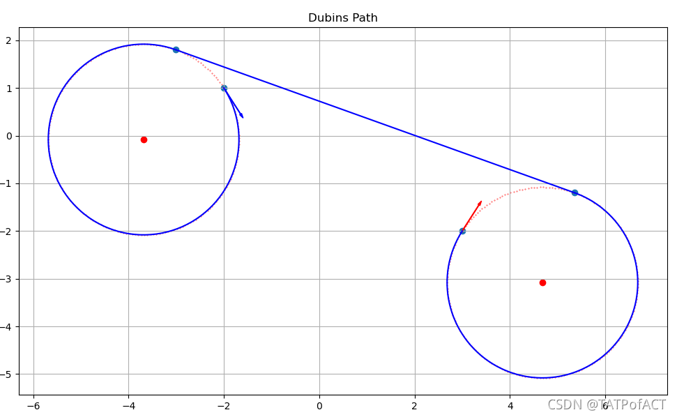
    path_point = Dubins_path(Pi=(-4., 1.), Pf=(5., -2.), alpha=-1, beta=1, ratio=2, tp="RSL")
    print(path_point)

效果

Julia代码实现

##########################################################
# 功能:
#   输入起止点的坐标,方向,转弯半径,曲线的种类，计算Dubins曲线
#
# 输入参数:
#   起点坐标:
#       Pi(x,y)
#   终点坐标:
#       Pf(x,y)
#   起点角度:
#       alpha(弧度)
#   终点角度:
#       beta(弧度)
#   转弯半径:
#       ratio
#   曲线类型:
#       tp "RSR","LSL","RSL","LSR"
#       ( R顺时针 L逆时针 S直线 default："RSR" )
#
# 输出结果：三元组
#   切出点坐标posiA:[A_x,A_y]
#   切入点坐标posiB:[B_x,B_y]
#   三段距离dist lst:[dist1出发圆弧,dist2直线,dist3到达圆弧
#
# Author: jia-yf19@mails.tsinghua.edu.cn
# Date  : 2021.10.29
#
##########################################################
function Dubins_path(Pi,Pf,α,β,r,tp="SRS")
    # 坐标系变化
    Mtr_Move = [1. 0. -Pi[1]; 0. 1. -Pi[2]; 0. 0. 1.] # 平移
    temp_θ = -(atan(Pf[2] - Pi[2], Pf[1] - Pi[1]) + π)
    α_ = α + temp_θ
    β_ = β + temp_θ
    Mtr_Rotate = [cos(temp_θ) -sin(temp_θ) 0.; sin(temp_θ) cos(temp_θ) 0.; 0. 0. 1.] # 旋转
    Mtr_Length = [1. / r 0. 0.; 0. 1. / r 0.; 0. 0. 1.]  # 拉伸
    Mtr_Trans = Mtr_Length * Mtr_Rotate *Mtr_Move
    temp_res = Mtr_Trans * [Pi[1]; Pi[2]; 1]
    Pi_ = [temp_res[1, 1], temp_res[2, 1]]
    temp_res = Mtr_Trans * [Pf[1]; Pf[2]; 1]
    Pf_ = [temp_res[1, 1], temp_res[2, 1]]

    # 曲线计算
    if tp == "RSR"  # 双逆时针路线
        Φ1_x, Φ1_y = sin(α_), -cos(α_)          # 起点圆
        Φ2_x, Φ2_y = Pf_[1] + sin(β_), -cos(β_)   # 终点圆
        θ = atan(Φ2_y - Φ1_y, Φ2_x - Φ1_x)         # 圆心夹角
        ρ1 = (θ - α_) % (2.0 * π)            # 起点圆弧度
        ρ2 = hypot((Φ1_x - Φ2_x), (Φ1_y - Φ2_y))    # 直线长度
        ρ3 = (β_ - ρ1 - ρ2 - α_) % (2.0 * π)  # 终点圆弧度
        A_x, A_y = sin(α_) - sin(α_ + ρ1), -cos(α_) + cos(α_ + ρ1)          # 切出点
        B_x, B_y = Pf_[1] + sin(β_) - sin(α_ + ρ1), -cos(β_) + cos(α_ + ρ1)   # 切入点
    elseif tp == "LSL"  # 双顺时针路线
        Φ1_x, Φ1_y = -sin(α_), cos(α_)          # 起点圆
        Φ2_x, Φ2_y = Pf_[1] - sin(β_), cos(β_)    # 终点圆
        θ = atan(Φ2_y - Φ1_y, Φ2_x - Φ1_x)         # 圆心夹角
        ρ1 = (θ - α_) % (2.0 * π)            # 起点圆弧度
        ρ2 = hypot((Φ1_x - Φ2_x), (Φ1_y - Φ2_y))    # 直线长度
        ρ3 = (β_ - ρ1 - ρ2 - α_) % (2.0 * π)  # 终点圆弧度
        A_x, A_y = -sin(α_) + sin(α_ + ρ1), cos(α_) - cos(α_ + ρ1)          # 切出点
        B_x, B_y = Pf_[1] - sin(β_) + sin(α_ + ρ1), cos(β_) - cos(α_ + ρ1)    # 切入点
    elseif tp == "RSL"  # 八字交叉路线
        Φ1_x, Φ1_y = sin(α_), -cos(α_)          # 起点圆
        Φ2_x, Φ2_y = Pf_[1] - sin(β_), cos(β_)    # 终点圆
        θ = atan(Φ2_y - Φ1_y, Φ2_x - Φ1_x)         # 圆心夹角
        dis_Φ1Φ2 = hypot((Φ2_y - Φ1_y), (Φ2_x - Φ1_x))
        if dis_Φ1Φ2 < 2.0
            println("The geometry constraint is not satisfied!")
            return Nothing
        else
            θ_Φ1A = acos(2. / dis_Φ1Φ2)             # 圆1圆心和A夹角
            A_x, A_y = sin(α_) + cos(θ + θ_Φ1A), -cos(α_) + sin(θ + θ_Φ1A)          # 切出点
            B_x, B_y = Pf_[1] - sin(β_) - cos(θ + θ_Φ1A), cos(β_) - sin(θ + θ_Φ1A)   # 切入点
        end
    else  # "LSR" # 另一种八字交叉路线
        Φ1_x, Φ1_y = -sin(α_), cos(α_)          # 起点圆
        Φ2_x, Φ2_y = Pf_[1] + sin(β_), -cos(β_)   # 终点圆
        θ = atan(Φ2_y - Φ1_y, Φ2_x - Φ1_x)         # 圆心夹角
        dis_Φ1Φ2 = hypot((Φ2_y - Φ1_y), (Φ2_x - Φ1_x))
        if dis_Φ1Φ2 < 2.0
            println("The geometry constraint is not satisfied!")
            return Nothing
        else
            θ_Φ1A = acos(2. / dis_Φ1Φ2)             # 圆1圆心和A夹角
            A_x, A_y = -sin(α_) + cos(θ - θ_Φ1A), cos(α_) + sin(θ - θ_Φ1A)          # 切出点
            B_x, B_y = Pf_[1] + sin(β_) - cos(θ - θ_Φ1A), -cos(β_) - sin(θ - θ_Φ1A)   # 切入点
        end
    end

    # 逆变换
    Mtr_Trans_INV = inv(Mtr_Trans)
    temp_res = Mtr_Trans_INV * [A_x; A_y; 1]
    A_x, A_y = (temp_res[1, 1], temp_res[2, 1])
    temp_res = Mtr_Trans_INV * [B_x; B_y; 1]
    B_x, B_y = (temp_res[1, 1], temp_res[2, 1])
    temp_res = Mtr_Trans_INV * [Φ1_x; Φ1_y; 1]
    Φ1_x, Φ1_y = (temp_res[1, 1], temp_res[2, 1])
    temp_res = Mtr_Trans_INV * [Φ2_x; Φ2_y; 1]
    Φ2_x, Φ2_y = (temp_res[1, 1], temp_res[2, 1])

    dis_lst = [0., 0., 0.]  # 每一段的距离
    ati1, ati2 = atan(Pi[2] - Φ1_y, Pi[1] - Φ1_x), atan(A_y - Φ1_y, A_x - Φ1_x)
    if tp[1] == 'R' && ati1 < ati2
        ati1 += 2.0 * π
    elseif tp[1] == 'L' && ati1 > ati2
        ati1 -= 2.0 * π
    end
    dis_lst[1] = r * abs(ati1 - ati2)  # 切出弧长度
    dis_lst[2] = hypot((A_x - B_x), (A_y - B_y))  # 直线段距离
    atf1 = atan(Pf[2] - Φ2_y, Pf[1] - Φ2_x)
    atf2 = atan(B_y - Φ2_y, B_x - Φ2_x)
    if tp[end] == 'R' && atf2 < atf1
        atf2 += 2.0 * π
    elseif tp[end] == 'L' && atf2 > atf1
        atf2 -= 2.0 * π
    end
    dis_lst[3] = (r * abs(atf1 - atf2))  # 切入弧长度 

    return ([A_x, A_y], [B_x, B_y], dis_lst)  # 切出点,切入点,每一段的距离
end

@time path_point = Dubins_path((2., 1.), (3., 2.), -1, 1, 3, "RSL")
println(path_point)

相关链接