梯度下降 - 举例线性回归

1 什么是梯度下降？

1.1 现实中的梯度下降

梯度下降法的基本思想可以类比为一个下山的过程——每次朝着当前位置**最陡峭（求导）**的方向的前进，就能到达山底了。

1.2 微分

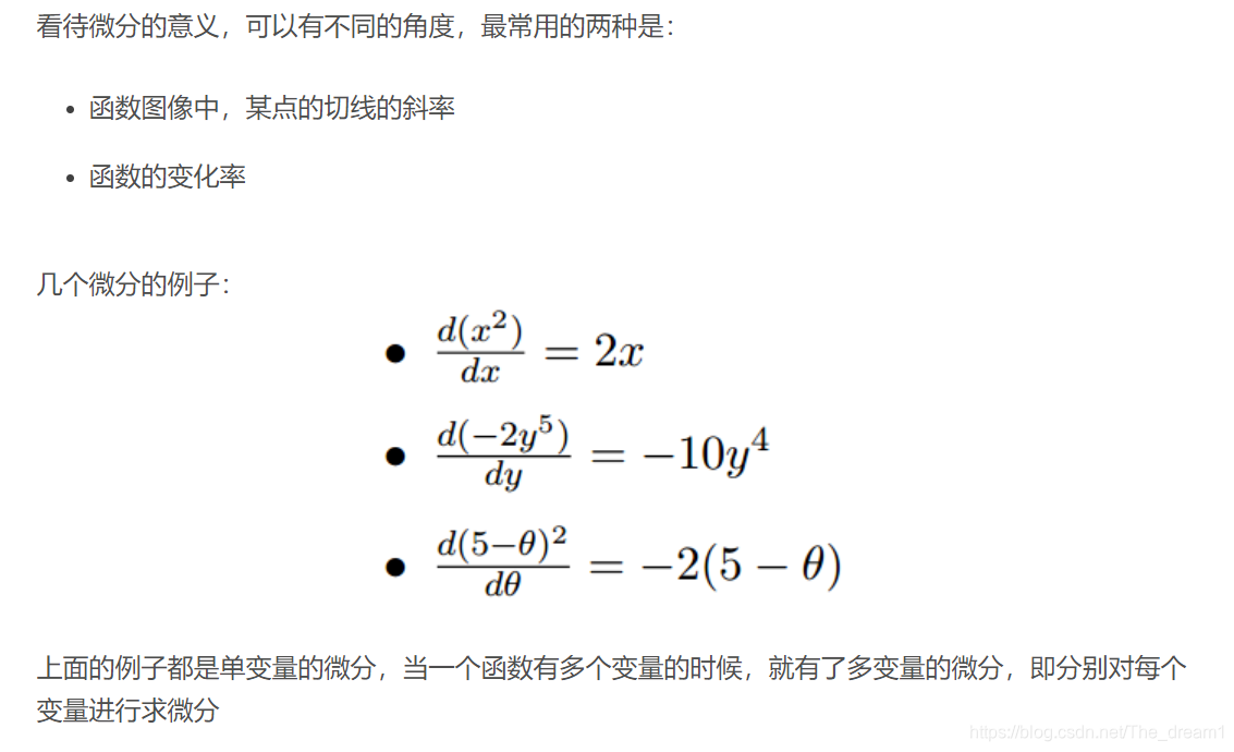
1.3 梯度

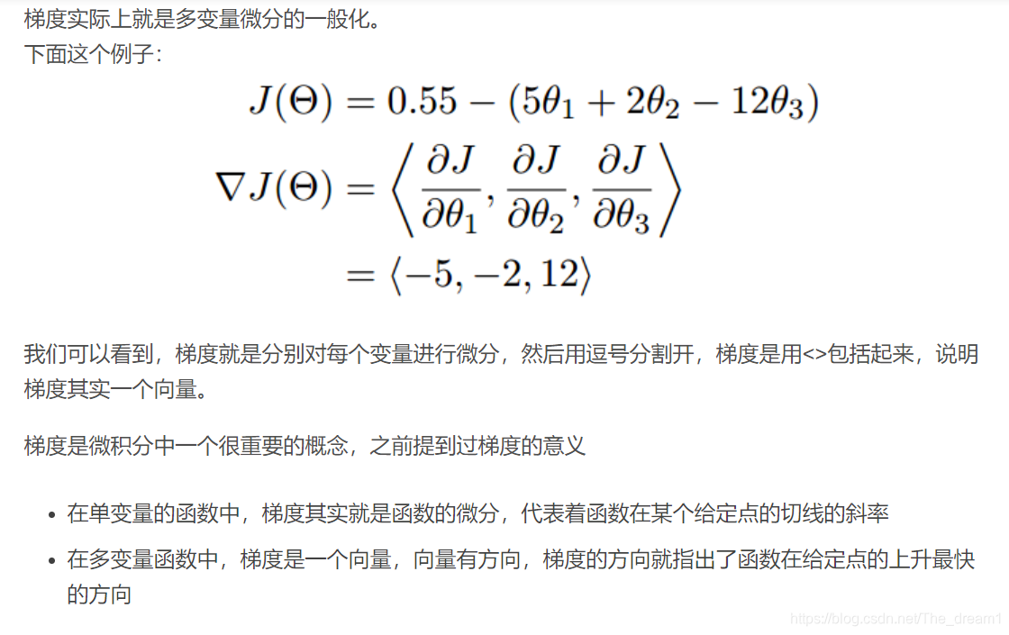
这也就说明了为什么我们需要千方百计的求取梯度！

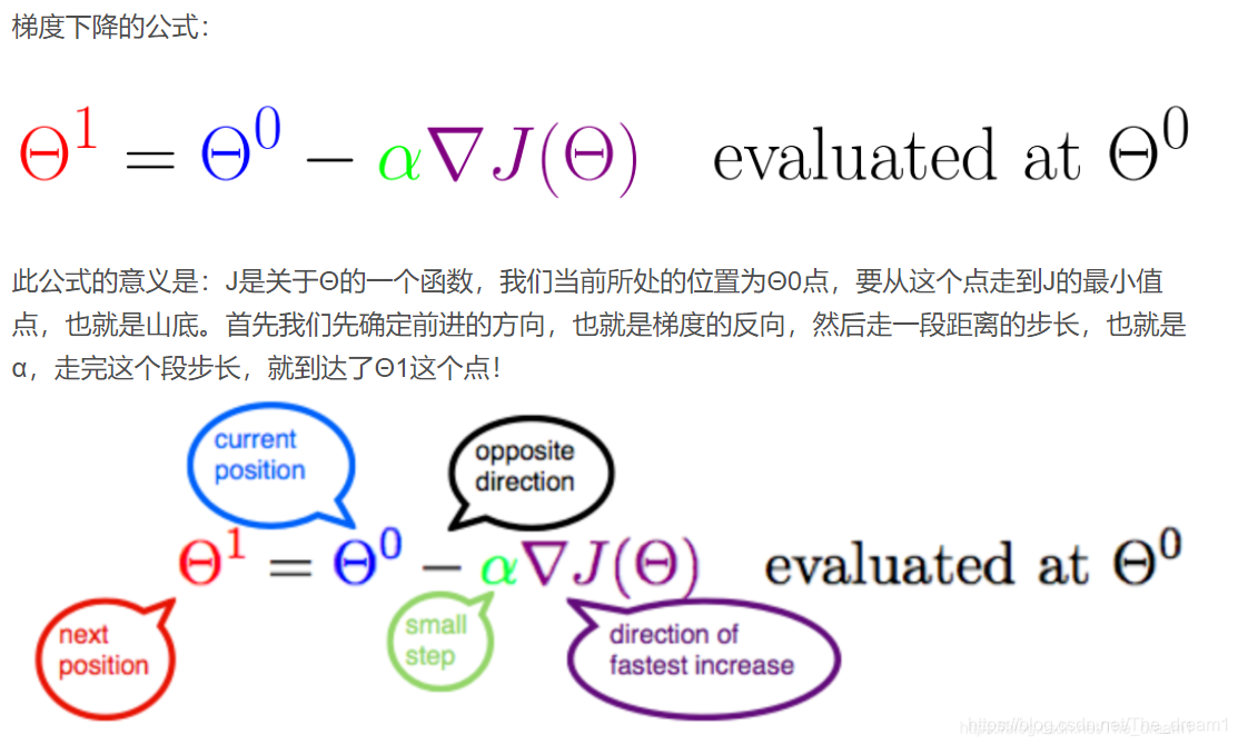
1.4 梯度下降算法的数学解释

梯度下降算法的数学解释

其中：

• α是什么？
  • 学习率/步长
• 为什么要梯度要乘以一个负号？
  • 梯度前加一个负号，就意味着朝着梯度相反的方向前进！

2 梯度下降算法的实例

我们已经基本了解了梯度下降算法的计算过程，那么我们就来看几个梯度下降算法的小实例，首先从单变量的函数开始

2.1 单变量函数的梯度下降

我们假设有一个单变量的函数

函数的微分

初始化，起点为

学习率为

根据梯度下降的计算公式

我们开始进行梯度下降的迭代计算过程：

如图，经过四次的运算，也就是走了四步，基本就抵达了函数的最低点，也就是山底

2.2 多变量函数的梯度下降

我们假设有一个目标函数

现在要通过梯度下降法计算这个函数的最小值。我们通过观察就能发现最小值其实就是 (0，0)点。但是接下来，我们会从梯度下降算法开始一步步计算到这个最小值！
我们假设初始的起点为：

初始的学习率为：

函数的梯度为：

进行多次迭代：

我们发现，已经基本靠近函数的最小值点

3 梯度下降算法的实现

3.1 引入依赖

import numpy as np
import matplotlib.pyplot as plt

3.2 导入数据（data.csv）

points = np.genfromtxt('data.csv', delimiter=',')

points[0,0]

# 提取points中的两列数据，分别作为x，y
x = points[:, 0]
y = points[:, 1]

# 用plt画出散点图
plt.scatter(x, y)
plt.show()

3.3 定义损失函数

# 损失函数是系数的函数，另外还要传入数据的x，y
def compute_cost(w, b, points):
    total_cost = 0
    M = len(points)
    
    # 逐点计算平方损失误差，然后求平均数
    for i in range(M):
        x = points[i, 0]
        y = points[i, 1]
        total_cost += ( y - w * x - b ) ** 2
    
    return total_cost/M

3. 4 定义模型的超参数

#对应学习率、w的权重、b的权重、迭代次数
alpha = 0.0001
initial_w = 0
initial_b = 0
num_iter = 10

3.5 定义核心梯度下降算法函数

def grad_desc(points, initial_w, initial_b, alpha, num_iter):
    w = initial_w
    b = initial_b
    # 定义一个list保存所有的损失函数值，用来显示下降的过程
    cost_list = []
    
    for i in range(num_iter):
        cost_list.append( compute_cost(w, b, points) )
        #这里用梯度下降求解参数
        w, b = step_grad_desc( w, b, alpha, points )
    
    return [w, b, cost_list]

def step_grad_desc( current_w, current_b, alpha, points ):
    sum_grad_w = 0
    sum_grad_b = 0
    M = len(points)
    
    # 对每个点，代入公式求和
    for i in range(M):
        x = points[i, 0]
        y = points[i, 1]
        sum_grad_w += ( current_w * x + current_b - y ) * x
        sum_grad_b += current_w * x + current_b - y
    
    # 用公式求当前梯度
    grad_w = 2/M * sum_grad_w
    grad_b = 2/M * sum_grad_b
    
    # 梯度下降，更新当前的w和b
    updated_w = current_w - alpha * grad_w
    updated_b = current_b - alpha * grad_b
    
    return updated_w, updated_b

3.6 测试：运行梯度下降算法计算最优的w和b

w, b, cost_list = grad_desc( points, initial_w, initial_b, alpha, num_iter )

print("w is: ", w)
print("b is: ", b)

cost = compute_cost(w, b, points)

print("cost is: ", cost)

plt.plot(cost_list)
plt.show()

3.7 画出拟合曲线

plt.scatter(x, y)
# 针对每一个x，计算出预测的y值
pred_y = w * x + b

plt.plot(x, pred_y, c='r')
plt.show()

参考：
https://www.cnblogs.com/pinard/p/5970503.html
https://www.jianshu.com/p/c7e642877b0e