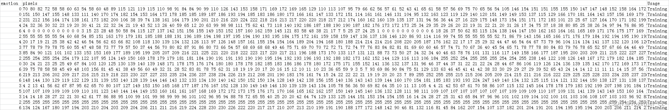
fer2013人脸表情数据实践

       Fer2013人脸表情数据集由35886张人脸表情图片组成，每张图片是由大小固定为48×48的灰度图像组成，共有7种表情，分别对应于数字标签0-6，具体表情对应的标签和中英文如下：

0 anger 生气
1 disgust 厌恶
2 fear 恐惧
3 happy 开心
4 sad 伤心
5 surprised 惊讶
6 normal 中性

      但是，数据集并没有直接给出图片，而是将表情、图片数据、用途的数据保存到csv文件中，如下图所示，

        这些数值型的数据可以直接读取、转化后存储为图像数据，这里我编写了对应的处理方法，代码实现如下所示：

def load2Image(filepath='fer2013.csv',saveDir='dataset/'):
    '''
    加载数据文件转化为图像数据存储本地
    '''
    data = pd.read_csv(filepath)
    pixels = data['pixels'].tolist()
    labels = data['emotion'].tolist()
    width, height = 48, 48
    faces = []
    for i in range(len(pixels)):
        one_pixel = pixels[i]
        one_label = str(labels[i])
        face = [int(pixel) for pixel in one_pixel.split(' ')]
        face = np.asarray(face).reshape(width, height)
        face = cv2.resize(face.astype('uint8'),(48,48))
        oneDir=saveDir+one_label+'/'
        if not os.path.exists(oneDir):
            os.makedirs(oneDir)
        one_path=oneDir+str(len(os.listdir(oneDir))+1)+'.jpg'
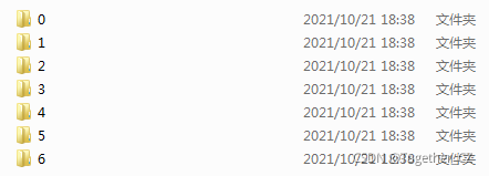
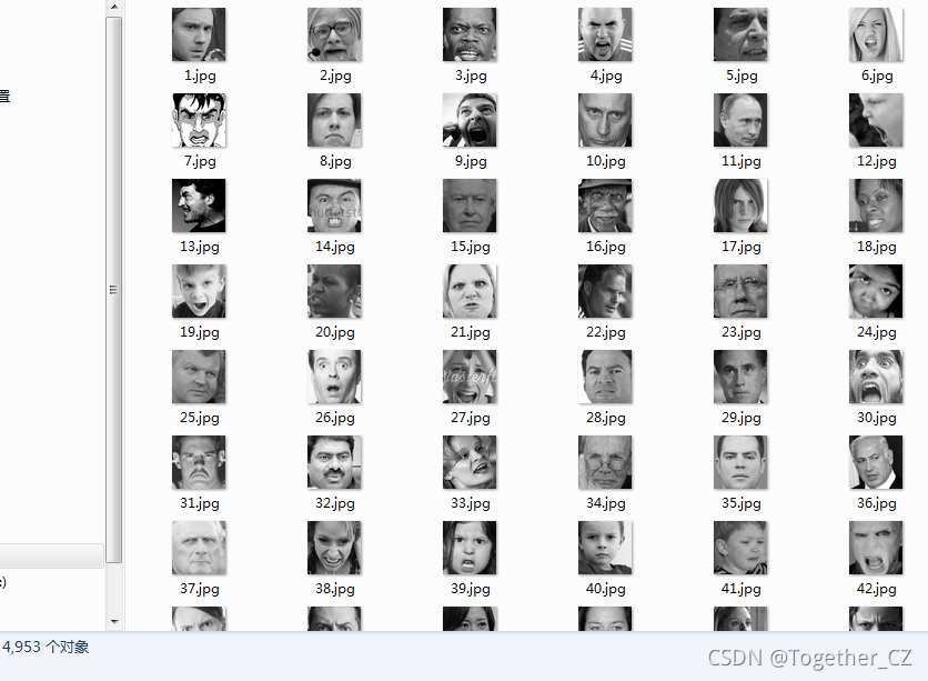
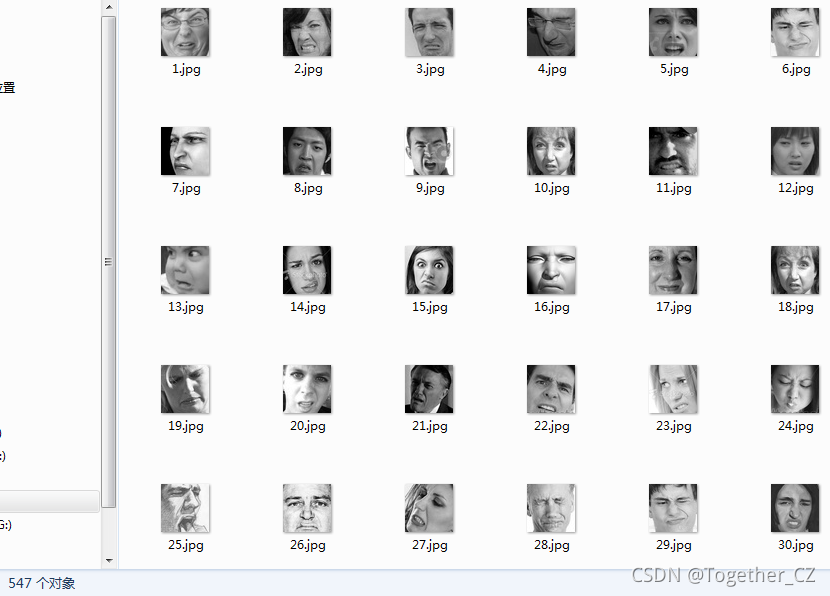
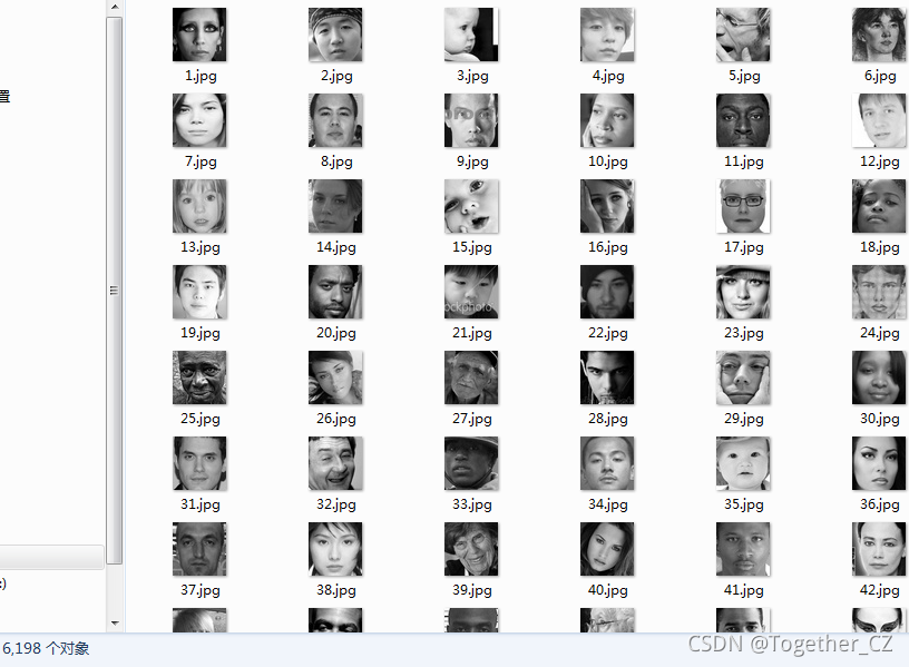
        cv2.imwrite(one_path,face)

         处理完成之后，数据集目录截图如下所示：

        0：

       1：

        2：

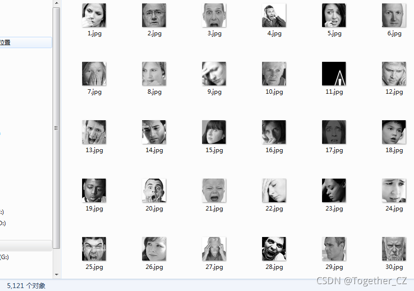
         3：

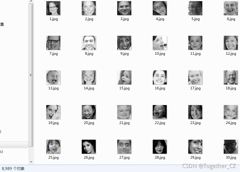
       4：

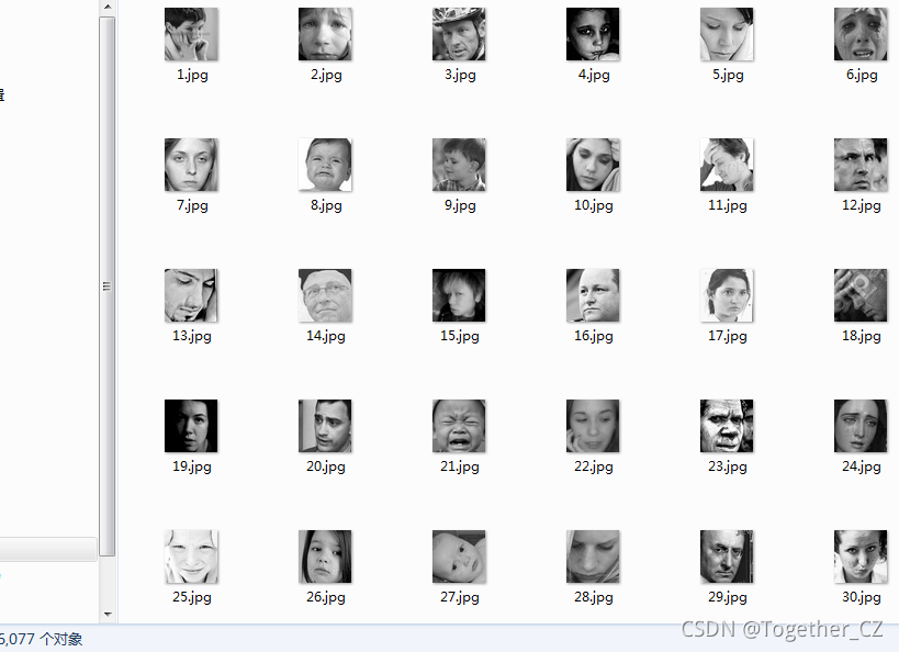
        5：

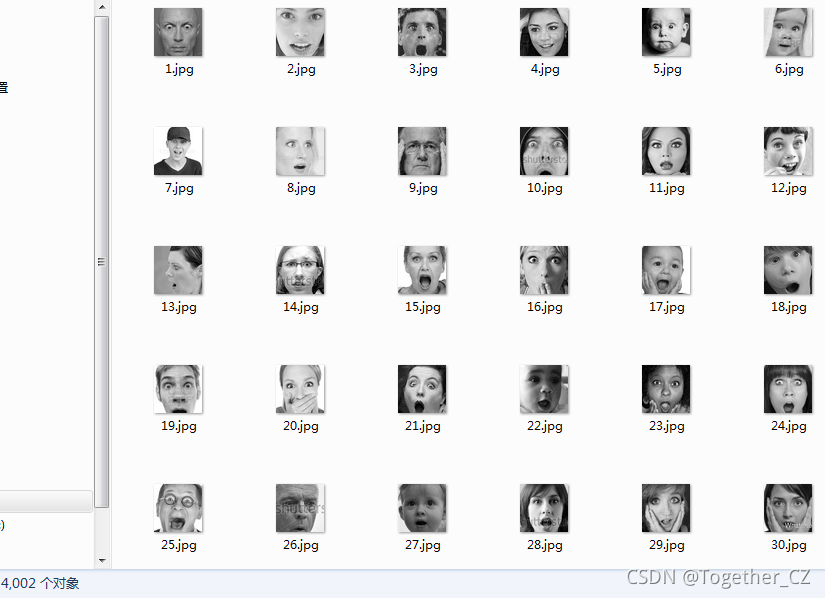
        6：

         可以看到：不同类别里面的数据集数量时不均衡的，尤其是类别1，数量只有其他类别的十分之一左右。

       初窥数据集之后，我们就开始处理数据集、搭建模型了，首先是数据集加载处理部分：

def loadData(filepath='fer2013.csv'):
    '''
    加载数据文件
    '''
    data = pd.read_csv(filepath)
    pixels = data['pixels'].tolist()
    width, height = 48, 48
    faces = []
    for pixel_sequence in pixels:
        face = [int(pixel) for pixel in pixel_sequence.split(' ')]
        face = np.asarray(face).reshape(width, height)
        face = cv2.resize(face.astype('uint8'),(48,48))
        faces.append(face.astype('float32'))
    faces = np.asarray(faces)
    faces = np.expand_dims(faces, -1)
    emotions = pd.get_dummies(data['emotion']).values
    return faces, emotions


def preprocess(x, v2=True):
    '''
    图像预处理
    '''
    x = x.astype('float32')
    x = x / 255.0
    if v2:
        x = x - 0.5
        x = x * 2.0
    return x

         读取原始的数据集之后对数据集图像数据进行了归一化处理，之后就可以输入到模型中了。由于深度学习模型所需数据较多，这里设计实现了图片生成器，这里也是为了尽可能减少数据不均衡带来的影响，数据生成器实现如下所示：

def imageGenerator(xtrain,ytrain,xtest,ytest):
    '''
    由于深度学习模型所需数据较多，这里设计实现了图片生成器
    '''
    train_datagen=ImageDataGenerator(
                                      rescale=1./255,
                                      rotation_range=40,
                                      width_shift_range=0.2,
                                      height_shift_range=0.2,
                                      shear_range=0.2,
                                      zoom_range=0.2,
                                      horizontal_flip=True,
                                      fill_mode='nearest')
    validation_datagen=ImageDataGenerator(rescale=1./255)
    train_generator=train_datagen.flow(xtrain, ytrain,batch_size)
    validation_generator=validation_datagen.flow(xtest, ytest,batch_size)
    return train_generator,validation_generator

        接下来是模型搭建部分，这里直接使用的是XCEPTION模型，Keras有了封装好的实现，如下所示：

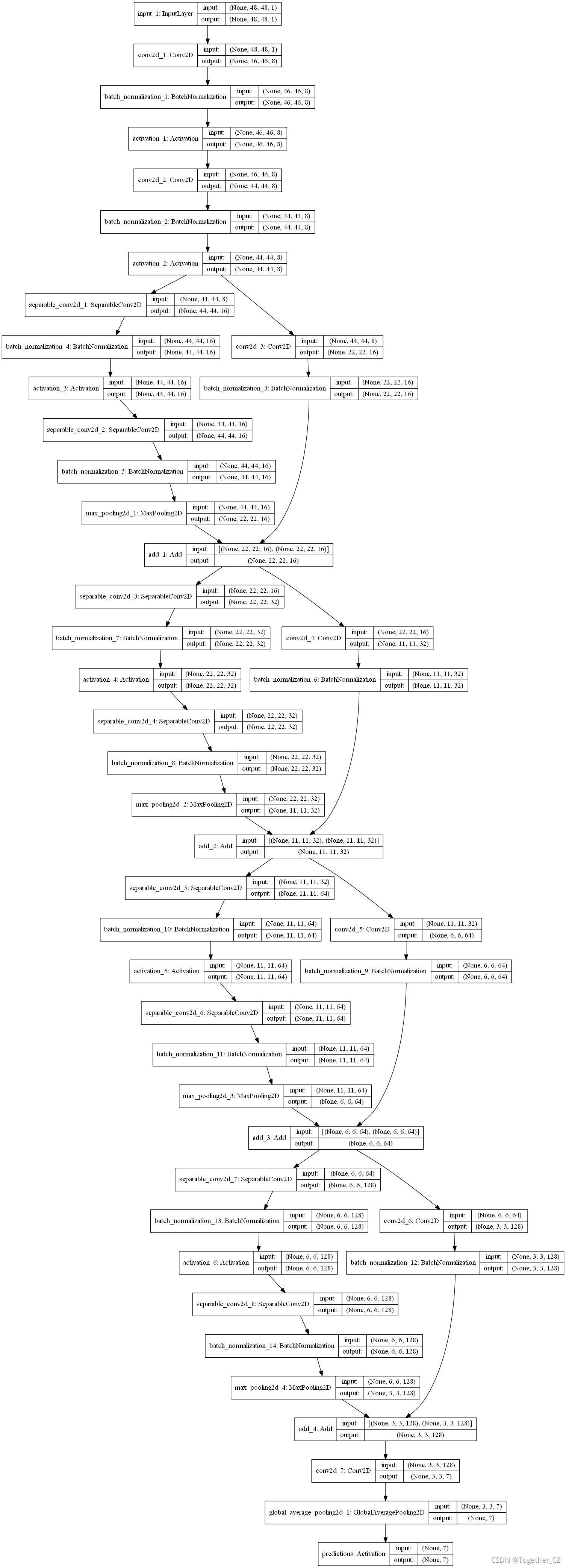
def initModel():
    '''
    resnet模型
    ''' 
    model = mini_XCEPTION(input_shape, num_classes)
    model.compile(optimizer='adam', loss='categorical_crossentropy',
                  metrics=['accuracy'])
    model.summary()
    return model

       完成模型的初始化搭建与数据生成器开发之后就可以进行对应的训练拟合了：

faces, emotions = loadData()
faces = preprocess(faces)
num_samples, num_classes = emotions.shape
xtrain, xtest,ytrain,ytest = train_test_split(faces, emotions,test_size=0.2,shuffle=True)

log_file_path = saveDir + 'training.log'
csv_logger = CSVLogger(log_file_path, append=False)
early_stop = EarlyStopping('val_loss', patience=patience)
reduce_lr = ReduceLROnPlateau('val_loss', factor=0.1,patience=int(patience/4), verbose=1)
checkpoint = ModelCheckpoint(filepath=saveDir+'model.h5',  monitor='loss', verbose=1, mode='min', 
                                 save_best_only = "True", period=1)
model=initModel()
#模型结构可视化
try:
    plot_model(model, to_file=saveDir+'model_structure.png', show_shapes=True)
except:
    pass
train_generator,test_generator=imageGenerator(xtrain,ytrain,xtest,ytest)
steps_per_epoch=len(xtrain) / batch_size
validation_steps=len(xtest) / batch_size
history=model.fit_generator(train_generator,epochs=100,steps_per_epoch=steps_per_epoch,
                            workers=16,callbacks=[checkpoint, csv_logger, early_stop, reduce_lr],
                            validation_data=test_generator,validation_steps=validation_steps)

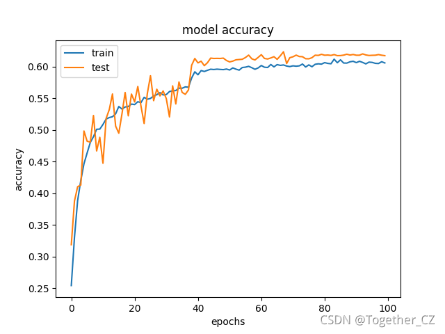
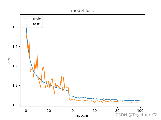
#训练数据曲线可视化
print(history.history.keys()) 
plt.clf()
plt.plot(history.history['acc'])
plt.plot(history.history['val_acc'])
plt.title('model accuracy')
plt.ylabel('accuracy')
plt.xlabel('epochs')
plt.legend(['train','test'], loc='upper left')
plt.savefig(saveDir+'train_validation_acc.png')
plt.clf()
plt.plot(history.history['loss'])
plt.plot(history.history['val_loss'])
plt.title('model loss')
plt.ylabel('loss')
plt.xlabel('epochs')
plt.legend(['train', 'test'], loc='upper left')
plt.savefig(saveDir+'train_validation_loss.png')
#保存模型结构+权重数据
model_json=model.to_json()
with open(saveDir+'structure.json','w') as f:
    f.write(model_json)
model.save_weights(saveDir+'weight.h5')
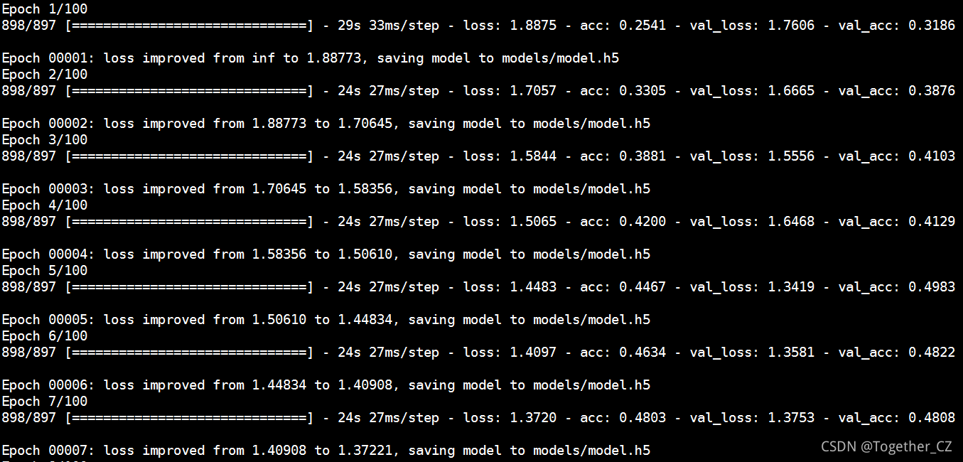
print('Model Save Success.........................................')

        这里我默认设置了100次迭代计算，模型启动输出如下所示：

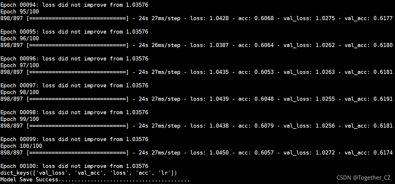
         训练结束如下所示：

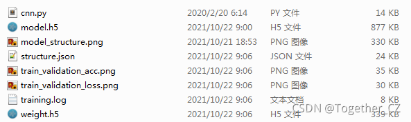
          结果目录如下所示：

       model_structure.png如下所示：

        train_validation_acc.png如下所示：

        train_validation_loss.png如下所示：

      到这里，本文的实践就结束了，后面有时间会补充一个实时计算模块，加载本地模型调用摄像头来对视频流进行实时计算分析。