R语言：关联规则可视化

关联规则可视化后各种参数的修改：点的大小、颜色、透明度修改、图例修改、网格删除等。

1.导入相关库

#导入相关库
library(arules) 
library(arulesViz)
library(RColorBrewer)
library(ggplot2)

2.加载数据集

rgroceries <- read.transactions("groceries.csv", format="basket", sep=",")

> summary(groceries)
transactions as itemMatrix in sparse format with
 9835 rows (elements/itemsets/transactions) and
 169 columns (items) and a density of 0.02609146 

most frequent items:
      whole milk other vegetables       rolls/buns             soda           yogurt 
            2513             1903             1809             1715             1372 
         (Other) 
           34055 

element (itemset/transaction) length distribution:
sizes
   1    2    3    4    5    6    7    8    9   10   11   12   13   14   15   16   17   18   19 
2159 1643 1299 1005  855  645  545  438  350  246  182  117   78   77   55   46   29   14   14 
  20   21   22   23   24   26   27   28   29   32 
   9   11    4    6    1    1    1    1    3    1 

   Min. 1st Qu.  Median    Mean 3rd Qu.    Max. 
  1.000   2.000   3.000   4.409   6.000  32.000 

includes extended item information - examples:
            labels
1 abrasive cleaner
2 artif. sweetener
3   baby cosmetics

构建关联规则

second.rules <- apriori(groceries,parameter = list(support = 0.025, confidence = 0.05))

> second.rules <- apriori(groceries,parameter = list(support = 0.025, confidence = 0.05))
Apriori

Parameter specification:
 confidence minval smax arem  aval originalSupport maxtime support minlen maxlen target  ext
       0.05    0.1    1 none FALSE            TRUE       5   0.025      1     10  rules TRUE

Algorithmic control:
 filter tree heap memopt load sort verbose
    0.1 TRUE TRUE  FALSE TRUE    2    TRUE

Absolute minimum support count: 245 

set item appearances ...[0 item(s)] done [0.00s].
set transactions ...[169 item(s), 9835 transaction(s)] done [0.01s].
sorting and recoding items ... [54 item(s)] done [0.00s].
creating transaction tree ... done [0.00s].
checking subsets of size 1 2 3 done [0.00s].
writing ... [96 rule(s)] done [0.00s].
creating S4 object  ... done [0.00s].

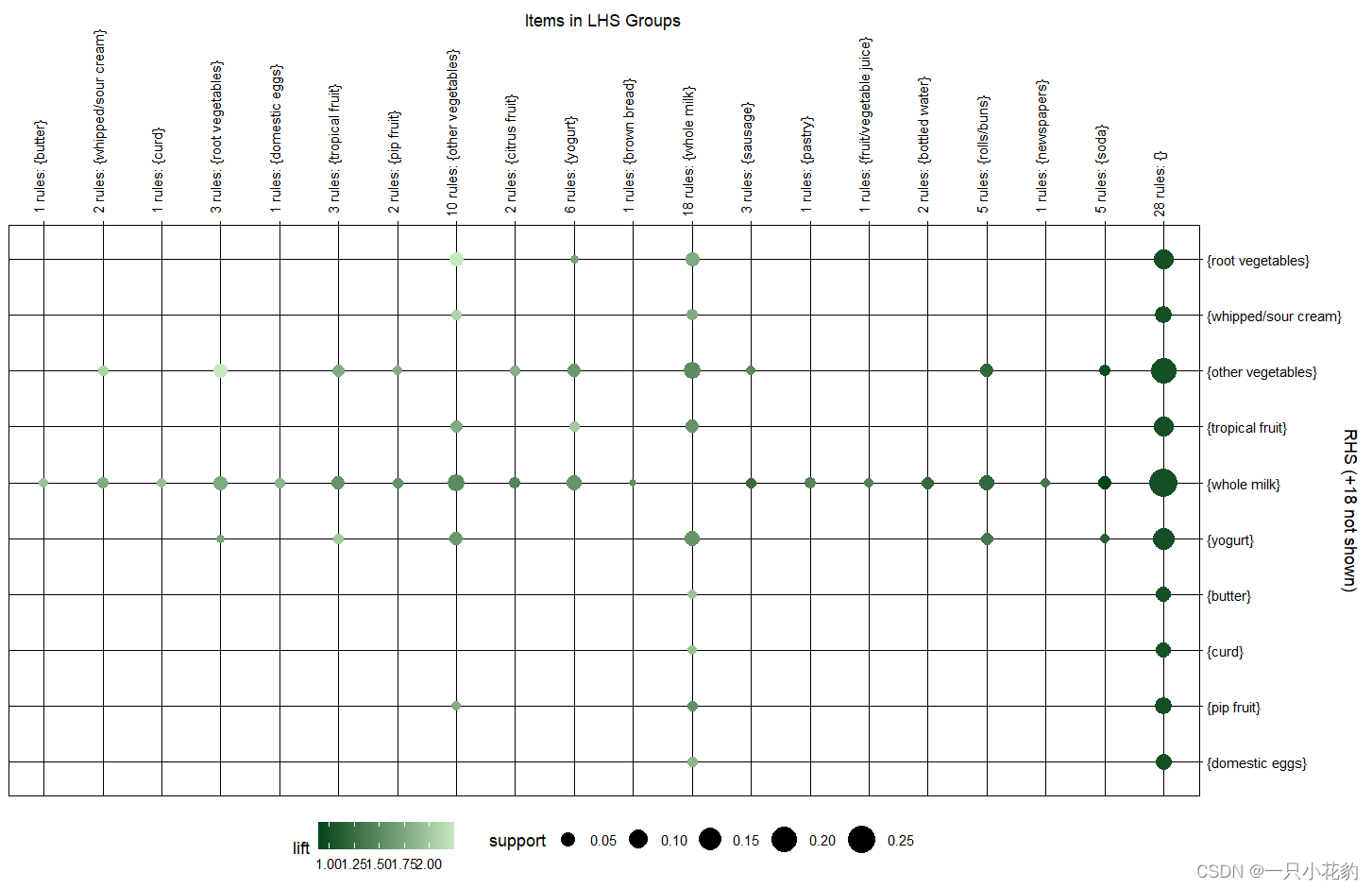
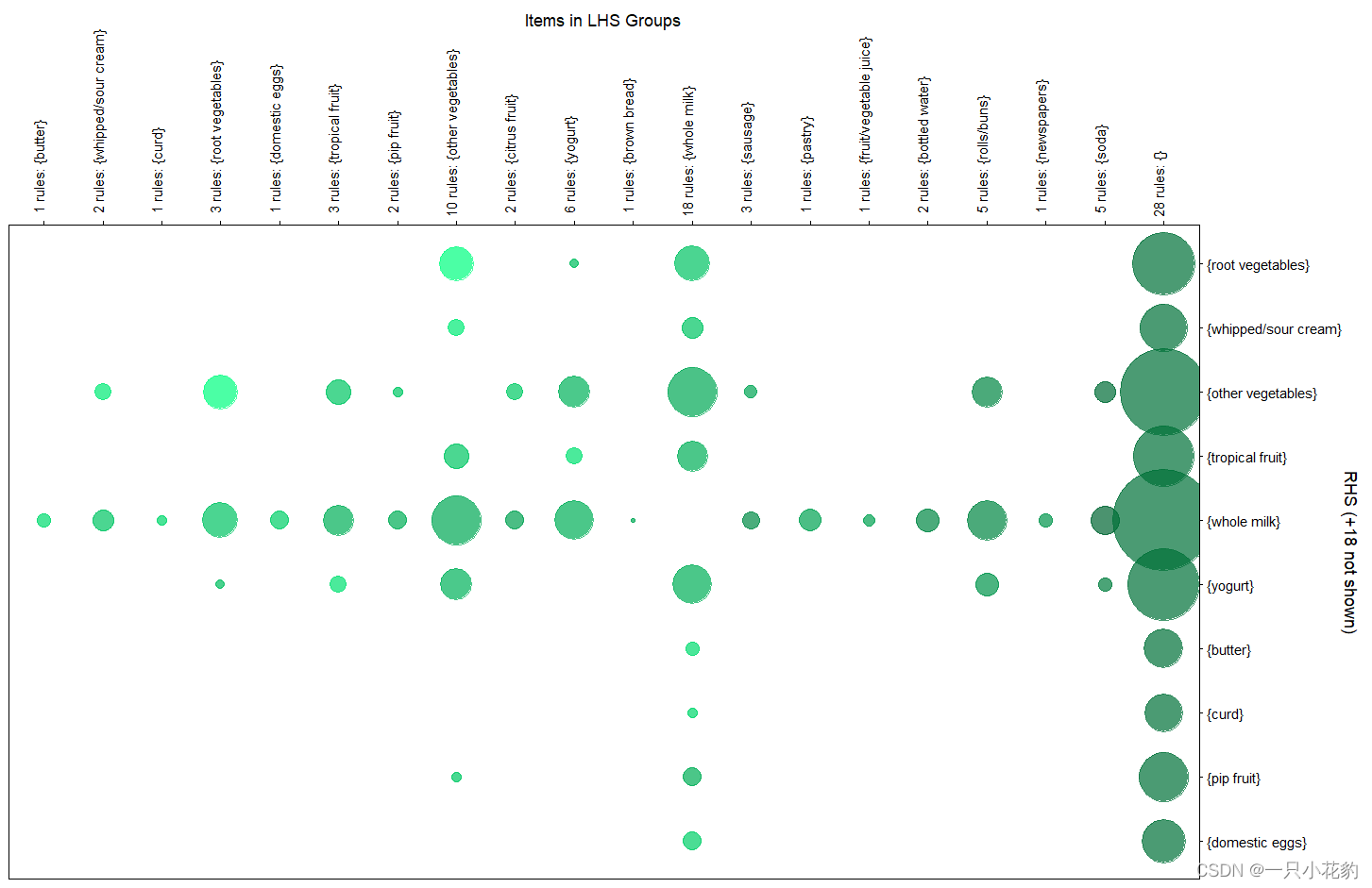
绘制关联规则矩阵

 plot(second.rules, method="grouped",engine = 'ggplot2',
             control=list(col = c(rev(brewer.pal(9, "Greens")[3]),rev(brewer.pal(9, "Greens")[7:9]))))

上述代码中，plot为实现关联规则可视化函数，这里engin参数为外部引擎，可以理解为在函数内调用其他包的功能，coltrol参数主要控制图的颜色等，这里颜色设置为绿色，成果图如下：

下面就是通过ggplot2对图片进行修改

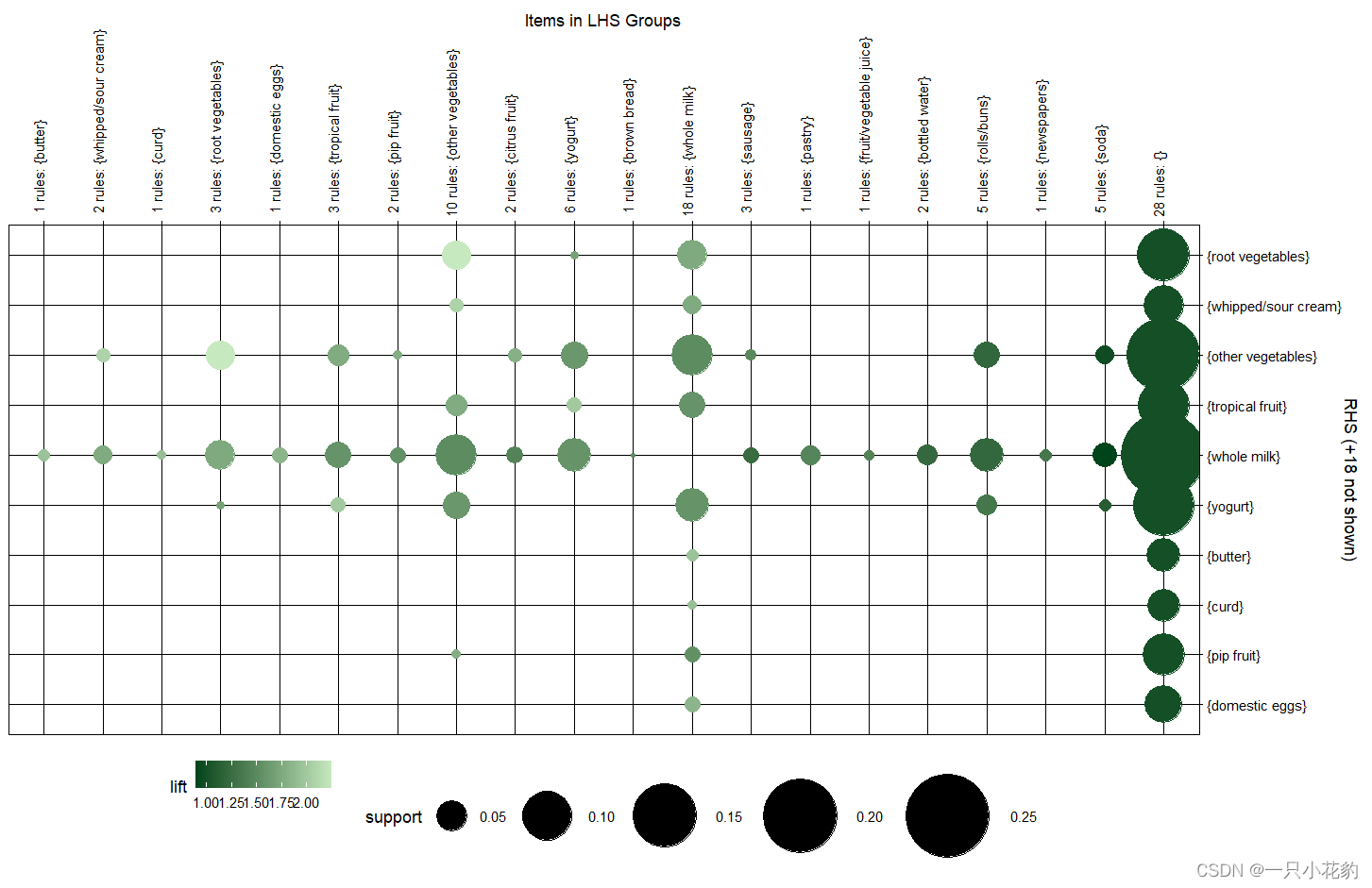
点的大小修改

由于关联规则矩阵初始时的点大小由置信度与支持度决定所以无法通过数据集进行自由的更改点的大小，不过可以通过ggplot的scale_size_continuous()函数去定位点，然后实现点大小的更改。

plot(second.rules, method="grouped",engine = 'ggplot2',
             control=list(col = c(rev(brewer.pal(9, "Greens")[3]),rev(brewer.pal(9, "Greens")[7:9]))))+
   scale_size_continuous(range = c(1,25))

其中range的值为c(n,m),n与m都为数字类型，表示点的大小在n到m间变化。
这里选择的范围为1:25效果如下：

可以看到图中的点已经明显增大，但需要注意的是，图例中的点也会随之增大，这是由于ggplot引擎，无发清晰的分别图与图例，为防止逐渐增大的图例使图片显得拥挤，这里直接去除图例，方法为ggplot的 theme()函数:

 plot(second.rules, method="grouped",engine = 'ggplot2',
             control=list(col = c(rev(brewer.pal(9, "Greens")[3]),rev(brewer.pal(9, "Greens")[7:9]))))+
   scale_size_continuous(range = c(1,25))+
    theme(legend.position = 'none')

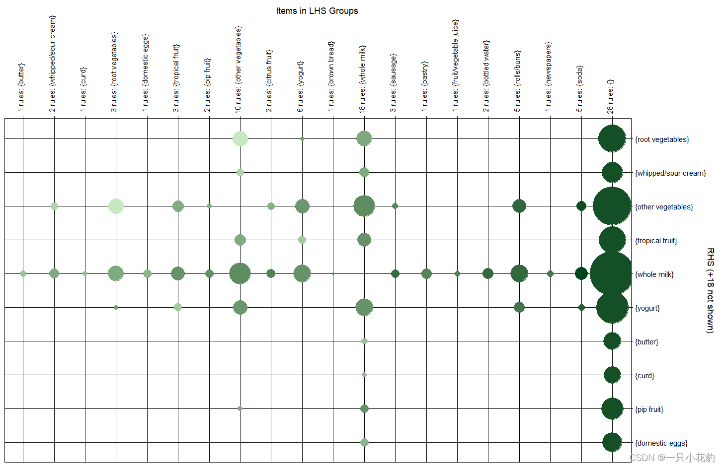
在函数theme(legend.position = ‘none’)中none为无图例，同样也可以改为图例在右边或左边，具体实现可以去查一下ggplot的theme函数这里不做过多演示。

透明度修改

目前图中的点虽然可以调整大小，不过相邻的点在增大后会相互覆盖，影响规则的判断，下面通过rgb()函数为点设置透明度，使点以堆叠的形式呈现：

 color <- c(rgb(0,255,128,180,maxColorValue = 255),rgb(0,102,51,180,maxColorValue = 255),rgb(0,102,51,180,maxColorValue = 255))
 plot(second.rules, method="grouped",engine = 'ggplot2',col = color)+
       scale_size_continuous(range = c(1,30))+#调整点的大小范围
       theme(legend.position = 'none') #去除图例为none

上述代码中使用的rgb()函数包含的参数为 rgb（红，绿，蓝，透明度，最大颜色值），其中颜色以数值呈现，某个值越大就越靠近哪个颜色，下面来看看成图效果：

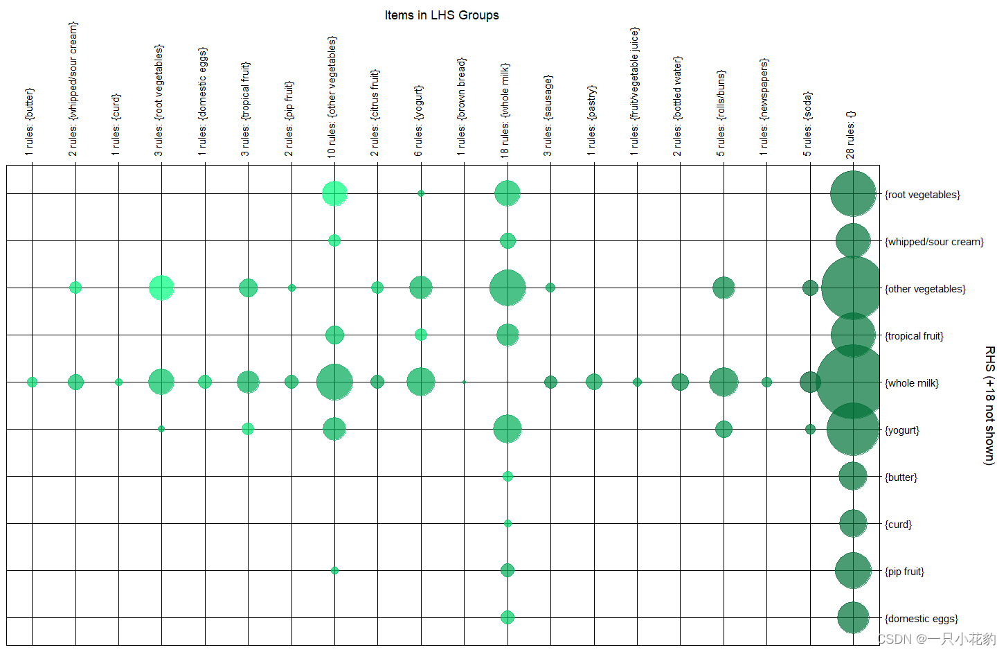
可以发现相邻的点已经呈现出透明堆叠的形态

网格线修改

网格线有时会让图显得乱一些，不够简洁，可以根据个人喜好进行去除，实现方法也是ggplot的去除网格线方法：theme(panel.grid = element_blank())
：

  plot(second.rules, method="grouped",engine = 'ggplot2',col = color)+
       scale_size_continuous(range = c(1,30))+#调整点的大小范围
       theme(panel.grid = element_blank())+#去除网格线
       theme(legend.position = 'none') #去除图例为none

以上便是本期全部的修改了，实际上大家应该不难发现，修改plot图的方法就是在调用ggplot之后使用ggplot的格式进行更改，所以其他功能也可以类比这这个案例进行实现，另外arulesViz 包还有另外两种关联规则的图，网状图和散点图，修改方法也同理。