回归——线性回归模型复现

回归——线性回归模型复现

问题重述

现在有一个二维空间中的点集$[x_i,y_i]$，需要使用如下线性模型拟合：
$$y=w\ast x+b$$
要求拟合误差尽可能小。对于所有的点$(x_i,y_i)$，误差用如下函数衡量：
$$loss=\sum (y_i-(w\ast x_i+b){)}^2$$
其中：

• $w\ast x_i+b$表示预测的值
• $y_i$表示真实的值
• $y_i-(w\ast x_i+b)$表示预测值与真实值的偏差，取平方使得每一项都为正数
• 最后将每一组$ (x_i,y_i)$的偏差求和即为总的偏差值

求解思路——梯度下降法

求解的目标是通过改变$w$和$b$，使得对于点集$[x_i,y_i]$计算出的$loss$函数的值最小。

根据导数的含义，我们知道$\frac{\partial loss}{\partial w}$表示当前状态下$w$微小的变化造成的$loss$变化量的多少，同理，$\frac{\partial loss}{\partial b}$表示当前状态下$b$微小的变化造成的$loss$变化量的多少，而$(\frac{\partial loss}{\partial w},\frac{\partial loss}{\partial b})$为函数$loss$的梯度，$loss$函数延负梯度方向下降最快

经过计算，我们可以得到：
$$\begin{gathered} \frac{\partial loss}{\partial w}=\sum 2\ast x_i\ast (y_i-(w\ast x_i+b)) \\ \frac{\partial loss}{\partial b}=\sum 2\ast (y_i-(w\ast x_i+b)) \end{gathered}$$
于是，我们可以沿着负梯度方向，通过如下公式不断更新$w$和$b$，使得$loss$以最快的速度不断减小直至局部最小值：
$$\begin{gathered} w_{new}=w_{old}-\alpha \ast \frac{\partial loss}{\partial w}=w_{old}-\alpha \ast \sum 2\ast x_i\ast (y_i-(w\ast x_i+b)) \\ {b}_{new}=b_{old}-\alpha \ast \frac{\partial loss}{\partial b}=b_{old}-\alpha \ast \sum 2\ast (y_i-(w\ast x_i+b)) \end{gathered}$$
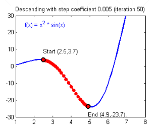
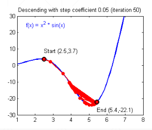
其中$\alpha$称为学习率（learningRate)，也就是沿负梯度方向每一次前进的“步伐长度”，如果$\alpha$选择太小将会导致下降速度过慢，需要迭代多次才能到达局部最小值点。如果$\alpha$选择过大将会导致步伐过大错过了局部最小值点，从而在最小值点附近震荡。

注意：

• 如果步伐足够小，则在不断逼近最小值点的过程中，每一次计算出的$\frac{\partial loss}{\partial w}$和$\frac{\partial loss}{\partial b}$都会不断减小，从而即使不用调整$\alpha$每次移动步伐也会不断减小，最终收敛到局部最小值点
  

• 如果步伐过大导致剧烈的震荡，每一次计算出的$\frac{\partial loss}{\partial w}$和$\frac{\partial loss}{\partial b}$都会增大，从而导致步伐进一步增大，震荡幅度不断增大。这是一个正反馈，最终导致$loss$达到无穷大
  

模型复现

数据的生成

使用软件:matlab

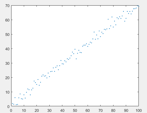
首先在matlab中使用$y=0.7\ast x+1.22+err$生成100个点的数据，其中$err$为一个服从正态分布$N(0,2)$的随机抖动。得到的点如下图所示：

之后将点的数据写入excel表格中

模型求解

编译环境：Pytorch3.7

语言：python

代码：

#coding=utf-8
import numpy as np
import xlrd

#读取excel文件的内容
class excel_read:
    def __init__(self, excel_path=r'data2.xlsx', encoding='utf-8', index=0):
        self.data = xlrd.open_workbook(excel_path)  ##获取文本对象
        self.table = self.data.sheets()[index]  ###根据index获取某个sheet
        self.rows = self.table.nrows  ##3获取当前sheet页面的总行数,把每一行数据作为list放到 list

    def get_data(self):
        result = []
        for i in range(self.rows):
            col = self.table.row_values(i)  ##获取每一列数据
            #print(col)
            result.append(col)
        #print(result)
        return result


#计算loss
def compute_error_for_line_given_points(b, w, points):
    totalError = 0
    for i in range(0, len(points)):
        x = points[i, 0]
        y = points[i, 1]
        totalError += (y - (w * x + b)) ** 2
    return totalError / float(len(points))

#延负梯度方向更新b和w
def step_gradient(b_current, w_current, points, learningRate):
    b_gradient = 0
    w_gradient = 0
    N = float(len(points))
    for i in range(0, len(points)):
        x = points[i, 0]
        y = points[i, 1]
        b_gradient += -(2 / N) * (y - ((w_current * x) + b_current))
        w_gradient += -(2 / N) * x * (y - ((w_current * x) + b_current))
    new_b = b_current - (learningRate * b_gradient)
    new_w = w_current - (learningRate * w_gradient)
    return [new_b, new_w]

#不断进行迭代
def gradient_descent_runner(points, starting_b, starting_w, learningRate, num_iterations):
    b = starting_b
    w = starting_w
    for i in range(num_iterations):
        b, w = step_gradient(b, w, np.array(points), learningRate)
    return [b, w]

#主程序
def run():
    #初始化
    points = np.array(excel_read().get_data())
    learningRate = 0.00005
    initial_b = 0
    initial_w = 0
    num_iterations = 100000
    #输出初始条件
    print("Starting at b={0},w={1},error={2}".format(initial_b, initial_w,
                                                     compute_error_for_line_given_points(initial_b, initial_w, points)))
    #计算、迭代
    print("Running")
    [b, w] = gradient_descent_runner(points, initial_b, initial_w, learningRate, num_iterations)
    #输出结果
    print("End at b={0},w={1},error={2} after {3} turns".format(b, w, compute_error_for_line_given_points(b,w, points),num_iterations))


if __name__ == '__main__':
    run()

选取学习率为0.0001,迭代次数为50000,得到结果为: