5.深度学习 ② 常用损失函数 2）

上一篇 pytorch 常用loss函数整理篇（一）介绍了以下几种常用Loss:

• L1 Loss/平均绝对误差（MAE）
• L2 Loss/均方误差（MSE）
• SmoothL1 Loss
• BCELoss和BCEWithLogitsLoss
• NLL Loss（ negative log likelihood loss）和CrossEntropy Loss

接下来继续介绍其余LOSS函数：

1.Dice Loss

1.1 Dice Loss简介

Dice Loss首先出现在论文V-Net: Fully Convolutional Neural Networks for
Volumetric Medical Image Segmentation中。其源于Dice coefficient，由Thorvald Sørensen和Lee Raymond Dice于1945年提出，用来度量两个集合的相似程度。
Dice coefficient有个别名是F1 score，二者是等价的。
$F_1=2\frac{1}{\frac{1}{P}+\frac{1}{R}}=\frac{2PR}{P+R}=\frac{2TP}{2TP+FP+FN}=\frac{2|X\cap Y|}{|X|+|Y|}=Dicecoefficient$
P和R分别为precision及recall。
Dice Loss 定义为：
$DL\left(p,\hat{p}\right)=1-\frac{2p\hat{p}+1}{p+\hat{p}+1}$，
其中：$p$为标签，$\hat{p}$为预测结果， p ∈ { 0 , 1 } p \in \{0,1\} p∈{0,1},$0\le \hat{p}\le 1$。
因此要对预测结果进行torch.sigmoid()操作，使之处于(0,1)；
多类别可以在类别方向torch.nn.functional.softmax()操作。
另外，在处理多标签分类时，要采用one_hot形式。
下面给出了其一种coding方式，需要说明的是，要注意预测及标签数据格式：
如果无batch_size，数据为$C\ast H\ast W$格式，则可以直接使用代码中的DiceLoss()；
若存在batch_size，数据为$batch\_size\ast C\ast H\ast W$格式，则需要对batch中各数据求得的Loss进行平均。否则求出的Dice Loss是不正确的。本人在项目实践中就出过类似错误。

1.2 Dice Loss编程实现

class DiceLoss(nn.Module):
	def __init__(self):
		super(DiceLoss, self).__init__()
 
	def	forward(self, input, target):
		N = target.size(0)
		smooth = 1
 
		input_flat = input.view(N, -1)
		target_flat = target.view(N, -1)
 
		intersection = input_flat * target_flat
 
		loss = 2 * (intersection.sum(1) + smooth) / (input_flat.sum(1) + target_flat.sum(1) + smooth)
		loss = 1 - loss.sum() / N
 
		return loss

if __name__ == "__main__":
   
#    input = torch.randn( 2, 3, 3)
#    input = torch.sigmoid(input)
#    target=torch.empty((2,3,3)).random_(2)
    input =torch.tensor([[[0.2656, 0.4492, 0.3135],
         [0.8917, 0.2472, 0.4546],
         [0.3573, 0.1485, 0.3700]],

        [[0.7022, 0.3999, 0.5945],
         [0.2945, 0.3459, 0.6240],
         [0.4438, 0.7022, 0.7051]]])
    target=torch.tensor([[[1., 0., 0.],
         [0., 0., 1.],
         [1., 0., 0.]],

        [[1., 0., 1.],
         [1., 1., 1.],
         [0., 1., 1.]]])
    loss=DiceLoss()
    
    res=loss(input,target)
    print(res)
    
    input_batch=torch.unsqueeze(input, 0)
    target=torch.unsqueeze(target, 0)   
    res=loss(input_batch,target)    
    print(res)

结果为：

tensor(0.3351)#2*3*3
tensor(0.3738)#加上batch_size 1,1*2*3*3

可以看出二者结果并不一致。
这里推荐github上的一种实现方式，以供参考：
hubutui/DiceLoss-PyTorch
Dice loss原理简图如下，详见链接:

1.3 其他

那么， Dice Loss是否会在各种情况下都work well呢？Dice-coefficient loss function vs cross-entropy帖子中给出了一些讨论，也被许多博客所引用：
The gradients of cross-entropy wrt the logits is something like p−t, where p is the softmax outputs and t is the target. Meanwhile, if we try to write the dice coefficient in a differentiable form: $\frac{2pt}{p^2+t^2}$ or $\frac{2pt}{p+t}$, then the resulting gradients wrt p are much uglier: $\frac{2t(t^2-p^2)}{(p^2+t^2{)}^2}$ and $\frac{2t^2}{(p+t{)}^2}$. It’s easy to imagine a case where both p and t are small, and the gradient blows up to some huge value. In general, it seems likely that training will become more unstable.
…class imbalance is typically taken care of simply by assigning loss multipliers to each class, such that the network is highly disincentivized to simply ignore a class which appears infrequently, so it’s unclear that Dice coefficient is really necessary in these cases.
具体有机会后续进一步论证吧。

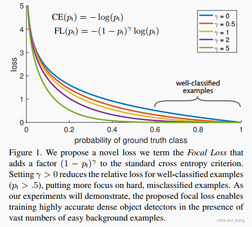
2.Focal Loss

2.1 Focal Loss简介

Focal Loss是在论文《Focal Loss for Dense Object Detection》首次提出。

它不仅可以解决正负样本不均衡的问题，也可以为难学习和容易学习样本分配不同的权重，达到down-weight easy examples and thus focus training on hard negatives，使得模型更关注于难学习的样本。这里仅讨论多分类的情况。

其公式为：
$\mathrm{FocalLoss}\left(\mathrm{X},Y\right)=\frac{1}{n}\sum _{i=1}^n-{\alpha }_t{(1-p_t)}^{\gamma }\log (p_t)$

核心观点见下图（来自原论文)：

2.2 Multi_class Focal Loss编程实现

代码实现参考了https://github.com/clcarwin/focal_loss_pytorch/blob/master/focalloss.py：

input tensor为one_hot形式的预测结果，其格式为batch_size∗channel∗height∗width，即$\mathrm{N}\ast \mathrm{C}\ast \mathrm{H}\ast \mathrm{W}$，target的输入格式为：$\mathrm{N}\ast \mathrm{H}\ast \mathrm{W}$。

首先对输入量进行LogSoftmax计算：

$\text{LogSoftmax}(X_i)=\log \left(\frac{\exp (X_i)}{{\sum }_j\exp (X_j)}\right)$，

然后按照2.1计算loss值。

import torch
import torch.nn as nn
import torch.nn.functional as F

class FocalLoss(nn.Module):
    def __init__(self, gamma=0, alpha=None, size_average=True):
        super(FocalLoss, self).__init__()
        self.gamma = gamma
        self.alpha = alpha
        self.size_average = size_average

    def forward(self, input, target):
        if input.dim() > 2:
            # N,C,H,W => N,C,H*W
            input = input.view(input.size(0), input.size(1), -1)
            input = input.transpose(1, 2)    # N,C,H*W => N,H*W,C
            input = input.contiguous().view(-1, input.size(2))   # N,H*W,C => N*H*W,C
        target = target.view(-1, 1)

        logpt = F.log_softmax(input, dim=1)
        logpt = logpt.gather(1, target)
        logpt = logpt.view(-1)
        pt = logpt.exp()

        if self.alpha is not None:
            at = self.alpha.gather(0, target.data.view(-1))
            logpt = logpt * at

        loss = -1 * (1-pt)**self.gamma * logpt
        if self.size_average:
            return loss.mean()
        else:
            return loss.sum()


if __name__ == "__main__":
    import random
    input = torch.rand(2, 10, 3, 4)*random.randint(1, 10)
    target = torch.rand(2, 3, 4)*10   # 1000 is classes_num
    target = target.long()
    print(FocalLoss(gamma=2, alpha=torch.rand(10))(input, target))

参考文献

1.What is “Dice loss” for image segmentation?
2.Lars’ Blog《Losses for Image Segmentation》
3.https://github.com/hubutui/DiceLoss-PyTorch/blob/master/loss.py
4.An overview of semantic image segmentation
5.https://github.com/clcarwin/focal_loss_pytorch/blob/master/focalloss.py