Basic regression: Predict fuel efficiency ------ TensorFlow

Basic_regression_Predict_fuel_efficiency

In a regression problem, the aim is to predict the output of a continuous value, like a price or a probability. Contrast this with a classification problem, where the aim is to select a class from a list of classes (for example, where a picture contains an apple or an orange, recognizing which fruit is in the picture).

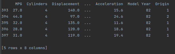
This tutorial uses the classic Auto MPG dataset and demonstrates how to build models to predict the fuel efficiency of the late-1970s and early 1980s automobiles. To do this, you will provide the models with a description of many automobiles from that time period. This description includes attributes like cylinders, displacement, horsepower, and weight.

url = 'http://archive.ics.uci.edu/ml/machine-learning-databases/auto-mpg/auto-mpg.data'
column_names = ['MPG', 'Cylinders', 'Displacement', 'Horsepower', 'Weight',
                'Acceleration', 'Model Year', 'Origin']

raw_dataset = pd.read_csv(url, names=column_names,
                          na_values='?', comment='\t',
                          sep=' ', skipinitialspace=True)

dataset = raw_dataset.copy()
print(dataset.tail())

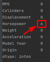
The dataset contains a few unknown values:
Drop those rows to keep this initial tutorial simple:

print(dataset.isna().sum())

dataset = dataset.dropna()

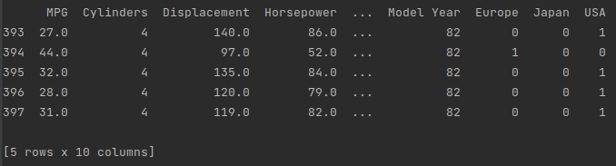
The “Origin” column is categorical, not numeric. So the next step is to one-hot encode the values in the column with pd.get_dummies
You can set up the tf.keras.Model to do this kind of transformation for you but that’s beyond the scope of this tutorial. Check out the Classify structured data using Keras preprocessing layers or Load CSV data tutorials for examples.

dataset['Origin'] = dataset['Origin'].map({1: 'USA', 2: 'Europe', 3: 'Japan'})
dataset = pd.get_dummies(dataset, columns=['Origin'], prefix='', prefix_sep='')
print(dataset.tail())

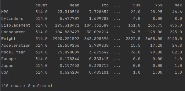
Let’s also check the overall statistics. Note how each feature covers a very different range:

print(train_dataset.describe().transpose())

Separate the target value—the “label”—from the features. This label is the value that you will train the model to predict.

train_features = train_dataset.copy()
test_features = test_dataset.copy()

train_labels = train_features.pop('MPG')
test_labels = test_features.pop('MPG')

It is good practice to normalize features that use different scales and ranges.
One reason this is important is because the features are multiplied by the model weights. So, the scale of the outputs and the scale of the gradients are affected by the scale of the inputs.
Although a model might converge without feature normalization, normalization makes training much more stable.

There is no advantage to normalizing the one-hot features—it is done here for simplicity. For more details on how to use the preprocessing layers, refer to the Working with preprocessing layers guide and the Classify structured data using Keras preprocessing layers tutorial.

The tf.keras.layers.Normalization is a clean and simple way to add feature normalization into your model.
The first step is to create the layer:

normalizer = tf.keras.layers.Normalization(axis=-1)

Then, fit the state of the preprocessing layer to the data by calling Normalization.adapt:

normalizer.adapt(np.array(train_features))

Calculate the mean and variance, and store them in the layer:

print(normalizer.mean.numpy())

When the layer is called, it returns the input data, with each feature independently normalized:

first = np.array(train_features[:1])

with np.printoptions(precision=2, suppress=True):
  print('First example:', first)
  print()
  print('Normalized:', normalizer(first).numpy())

The number of inputs can either be set by the input_shape argument, or automatically when the model is run for the first time

Mean squared error (MSE) (tf.losses.MeanMeanSquaredError) and mean absolute error (MAE) (tf.losses.MeanAbsoluteError) are common loss functions used for regression problems. MAE is less sensitive to outliers. Different loss functions are used for classification problems.

When numeric input data features have values with different ranges, each feature should be scaled independently to the same range

Overfitting is a common problem for DNN models, though it wasn’t a problem for this tutorial. Visit the Overfit and underfit tutorial for more help with this

import matplotlib.pyplot as plt
import numpy as np
import pandas as pd
import seaborn as sns

# Make NumPy printouts easier to read.
np.set_printoptions(precision=3, suppress=True)

import tensorflow as tf

from tensorflow import keras
from tensorflow.keras import layers

print(tf.__version__)

url = 'http://archive.ics.uci.edu/ml/machine-learning-databases/auto-mpg/auto-mpg.data'
column_names = ['MPG', 'Cylinders', 'Displacement', 'Horsepower', 'Weight',
                'Acceleration', 'Model Year', 'Origin']

raw_dataset = pd.read_csv(url, names=column_names,
                          na_values='?', comment='\t',
                          sep=' ', skipinitialspace=True)

dataset = raw_dataset.copy()
print(dataset.tail())

print(dataset.isna().sum())

dataset = dataset.dropna()
dataset['Origin'] = dataset['Origin'].map({1: 'USA', 2: 'Europe', 3: 'Japan'})
dataset = pd.get_dummies(dataset, columns=['Origin'], prefix='', prefix_sep='')
print(dataset.tail())

train_dataset = dataset.sample(frac=0.8, random_state=0)
test_dataset = dataset.drop(train_dataset.index)

print(train_dataset.describe().transpose())

train_features = train_dataset.copy()
test_features = test_dataset.copy()

train_labels = train_features.pop('MPG')
test_labels = test_features.pop('MPG')

print(train_dataset.describe().transpose()[['mean', 'std']])

normalizer = tf.keras.layers.Normalization(axis=-1)
normalizer.adapt(np.array(train_features))
print(normalizer.mean.numpy())

first = np.array(train_features[:1])

with np.printoptions(precision=2, suppress=True):
    print('First example:', first)
    print()
    print('Normalized:', normalizer(first).numpy())

horsepower = np.array(train_features['Horsepower'])

horsepower_normalizer = layers.Normalization(input_shape=[1, ], axis=None)
horsepower_normalizer.adapt(horsepower)

horsepower_model = tf.keras.Sequential([
    horsepower_normalizer,
    layers.Dense(units=1)
])

print(horsepower_model.summary())
print(horsepower_model.predict(horsepower[:10]))

horsepower_model.compile(
    optimizer=tf.optimizers.Adam(learning_rate=0.1),
    loss='mean_absolute_error')

history = horsepower_model.fit(
    train_features['Horsepower'],
    train_labels,
    epochs=100,
    # Suppress logging.
    verbose=0,
    # Calculate validation results on 20% of the training data.
    validation_split=0.2)

hist = pd.DataFrame(history.history)
hist['epoch'] = history.epoch
print(hist.tail())


def plot_loss(history):
    plt.plot(history.history['loss'], label='loss')
    plt.plot(history.history['val_loss'], label='val_loss')
    plt.ylim([0, 10])
    plt.xlabel('Epoch')
    plt.ylabel('Error [MPG]')
    plt.legend()
    plt.grid(True)
    plt.show()


plot_loss(history)

test_results = {}

test_results['horsepower_model'] = horsepower_model.evaluate(
    test_features['Horsepower'],
    test_labels, verbose=0)

linear_model = tf.keras.Sequential([
    normalizer,
    layers.Dense(units=1)
])

linear_model.compile(
    optimizer=tf.optimizers.Adam(learning_rate=0.1),
    loss='mean_absolute_error')

history = linear_model.fit(
    train_features,
    train_labels,
    epochs=100,
    # Suppress logging.
    verbose=0,
    # Calculate validation results on 20% of the training data.
    validation_split=0.2)

plot_loss(history)

test_results['linear_model'] = linear_model.evaluate(
    test_features, test_labels, verbose=0)


def build_and_compile_model(norm):
    model = keras.Sequential([
        norm,
        layers.Dense(64, activation='relu'),
        layers.Dense(64, activation='relu'),
        layers.Dense(1)
    ])

    model.compile(loss='mean_absolute_error',
                  optimizer=tf.keras.optimizers.Adam(0.001))
    return model


dnn_horsepower_model = build_and_compile_model(horsepower_normalizer)

print(dnn_horsepower_model.summary())

history = dnn_horsepower_model.fit(
    train_features['Horsepower'],
    train_labels,
    validation_split=0.2,
    verbose=0, epochs=100)

plot_loss(history)

test_results['dnn_horsepower_model'] = dnn_horsepower_model.evaluate(
    test_features['Horsepower'], test_labels,
    verbose=0)

dnn_model = build_and_compile_model(normalizer)
print(dnn_model.summary())

history = dnn_model.fit(
    train_features,
    train_labels,
    validation_split=0.2,
    verbose=0, epochs=100)

plot_loss(history)

test_results['dnn_model'] = dnn_model.evaluate(test_features, test_labels, verbose=0)

print(pd.DataFrame(test_results, index=['Mean absolute error [MPG]']).T)

从上图的预测结果可以发现， dnn_model 的效果最好

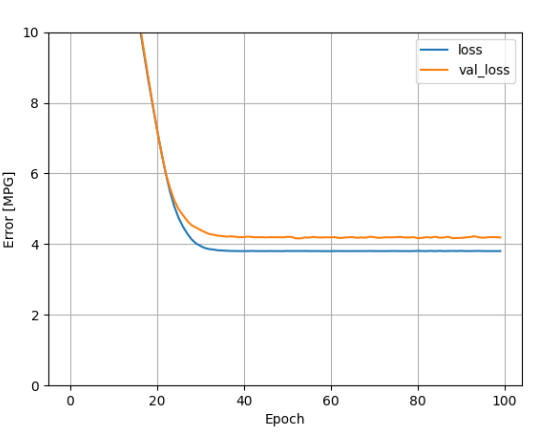
horsepower_model 的训练 log 图

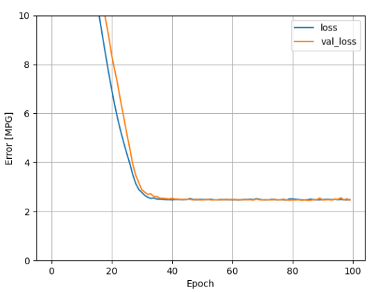
linear_model 的训练 log 图

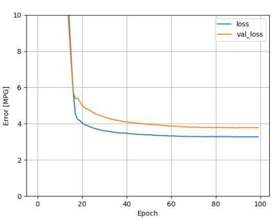
dnn_horsepower_model 的训练 log 图

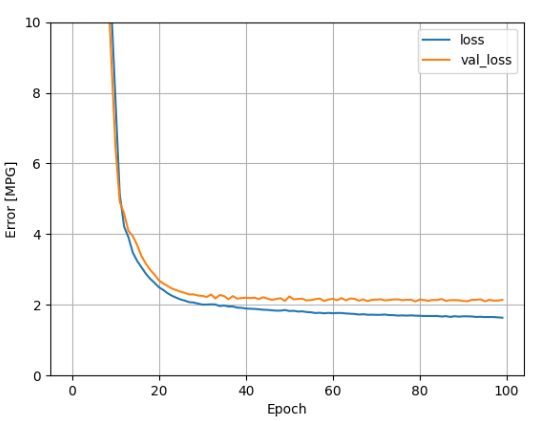
dnn_model 的训练 log 图