


前言
你好! 这是我第二篇学习PyTorch的笔记,通过一些案例来进行学习,防止自己忘记在这里记录一下,要是发现有什么可以改进的地方请一定告诉我啦~
开始学习
首先 本文主要讲解两个主要特征
- An n-dimensional Tensor, similar to numpy but can run on GPUs
一个和Numpy很相似的N维度的张量,但是它运行在GPU上- Automatic differentiation for building and training neural networks
可以自动分类的的神经网络构建和训练
这里我们使用全连接的Relu网络来作为我们的运行示例,这个网络具有单个隐藏层,并通过梯度下降法来进行训练,通过降低测试数据和真实数据的误差来最终实现随机数据的预测。
张量
这里先做一个热身,我们先用numpy来构建一个神经网络
Numpy 提供了一个 n 维数组对象,以及用于操作这些数组的许多函数。Numpy 是科学计算的通用框架;它不知道如何应对计算图形、深度学习或梯度。但是,我们可以轻松地使用 numpy 将双层网络用于随机数据,通过使用 numpy 运算手动实现神经网络的正向和反向传递:
# -*- coding: utf-8 -*-
import numpy as np

# N is batch size; D_in is input dimension;
# H is hidden dimension; D_out is output dimension.
# N是Batch Size,即一次训练所选取的样本数。
N, D_in, H, D_out = 64, 1000, 100, 10

# Create random input and output data
x = np.random.randn(N, D_in)
y = np.random.randn(N, D_out)

# Randomly initialize weights
w1 = np.random.randn(D_in, H)
w2 = np.random.randn(H, D_out)

# 学习率设置
learning_rate = 1e-6
for t in range(500):
    # Forward pass: compute predicted y
    h = x.dot(w1)
    h_relu = np.maximum(h, 0)
    y_pred = h_relu.dot(w2)

    # Compute and print loss
    loss = np.square(y_pred - y).sum()
    print(t, loss)

    # Backprop to compute gradients of w1 and w2 with respect to loss
    grad_y_pred = 2.0 * (y_pred - y)
    grad_w2 = h_relu.T.dot(grad_y_pred)
    grad_h_relu = grad_y_pred.dot(w2.T)
    grad_h = grad_h_relu.copy()
    grad_h[h < 0] = 0
    grad_w1 = x.T.dot(grad_h)

    # Update weights
    w1 -= learning_rate * grad_w1
    w2 -= learning_rate * grad_w2
代码解析:
这段代码展示了一个三层神经网络的构建和使用梯度下降运算的过程,先设定了选取样本数、输入维度大小、隐藏大小、输出维度大小分别为64,1000,100,10。
w1 = np.random.randn(D_in, H)
w2 = np.random.randn(H, D_out)
根据代码可知到权重参数矩阵w1为 (1000,100),w2为 (100,10),学习率为10-6
然后for循环500次来进行迭代,前行传播的过程时不断的矩阵乘法
最终得到的Y_pred的大小为(batch_size,10)
损失函数为误差的平方之和(这里借用大佬一张图)

所以在反向传播第一步,输出层的梯度为’grad_y_pred = 2.0 * (y_pred - y)
根据链式求导法则,隐层的梯度为grad_w2 = h_relu.T.dot(grad_y_pred)
Tensor 来实现神经网络
. Numpy 是一个伟大的框架,但它不能利用 GPU 来加速其数值计算。对于现代深度神经网络,GPU 通常提供50 倍或更高的加速,因此不幸的是,numpy 不足以用于深度学习。
在这里,我们介绍最基本的PyTorch概念:Tensor。PyTorch Tensor 在概念上与矩阵或是数组相同:Tensor 是一个 n 维数组,PyTorch 提供了许多函数来在这些 Tensors 上操作。Tensors 不仅可以跟踪计算图形和梯度,它们还作为科学计算的通用工具也很有用。
与numpy不同,PyTorch Tensors 可以利用 GPU 来加速其数值计算。要在 GPU 上运行 PyTorch Tensor,只需将其转换为新的数据类型即可。
我们使用 PyTorch Tensors 来将双层网络用于随机数据。与上面的数值示例一样,我们需要手动实现通过网络的正向和向后传递:
# -*- coding: utf-8 -*-
import torch
dtype = torch.float
device = torch.device("cpu")
# device = torch.device("cuda:0") # Uncomment this to run on GPU
# N is batch size; D_in is input dimension;
# H is hidden dimension; D_out is output dimension.
N, D_in, H, D_out = 64, 1000, 100, 10
# Create random input and output data
x = torch.randn(N, D_in, device=device, dtype=dtype)
y = torch.randn(N, D_out, device=device, dtype=dtype)
# Randomly initialize weights
w1 = torch.randn(D_in, H, device=device, dtype=dtype)
w2 = torch.randn(H, D_out, device=device, dtype=dtype)
learning_rate = 1e-6
for t in range(500):
# Forward pass: compute predicted y
h = x.mm(w1)
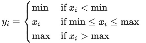
h_relu = h.clamp(min=0)
y_pred = h_relu.mm(w2)
# Compute and print loss
loss = (y_pred - y).pow(2).sum().item()
if t % 100 == 99:
print(t, loss)
# Backprop to compute gradients of w1 and w2 with respect to loss
grad_y_pred = 2.0 * (y_pred - y)
grad_w2 = h_relu.t().mm(grad_y_pred)
grad_h_relu = grad_y_pred.mm(w2.t())
grad_h = grad_h_relu.clone()
grad_h[h < 0] = 0
grad_w1 = x.t().mm(grad_h)
# Update weights using gradient descent
w1 -= learning_rate * grad_w1
w2 -= learning_rate * grad_w2
这里的relu使用的clamp函数
感觉很繁琐?看看自动求导机制吧
看了上面的例子,我们必须手动实现神经网络每个前向和后向的传播运算,对于小型双层神经网络,这不是什么难事,但是在面对大型的复杂网络时,这个运算将变得非常麻烦。
因此,我可以使用自动求导机制来自动计算神经网络中的反向传播,Pytorch中的autograd包提供了此功能,使用自动求导时,你的网络的前向传播通道会定义一个计算图(computational graph),图中的节点(node)是Tensors,即数据,边(edge)将会是根据输入Tensor来产生输出Tensor的函数方法。这个图的反向传播将会允许你很轻松地去计算梯度。
这个听起来复杂,但是实际操作非常简单。我们把PyTorch Tensors打包到Variable 对象中,一个Variable代表一个计算图中的节点。如果x是一个Variable,那么x. data 就是一个Tensor 。并且x.grad是另一个Variable,该Variable保持了x相对于某个标量值得梯度。
PyTorch的Variable具有与PyTorch Tensors相同的API。差不多所有适用于Tensor的运算都能适用于Variables。区别在于,使用Variables定义一个计算图,令我们可以自动计算梯度。
下面我们使用PyTorch 的Variables和自动梯度来执行我们的两层的神经网络。我们不再需要手动执行网络的反向通道了。
# -*- coding: utf-8 -*-
import torch

dtype = torch.float
device = torch.device("cpu")
# device = torch.device("cuda:0") # Uncomment this to run on GPU

# N is batch size; D_in is input dimension;
# H is hidden dimension; D_out is output dimension.
N, D_in, H, D_out = 64, 1000, 100, 10

# Create random Tensors to hold input and outputs.
# Setting requires_grad=False indicates that we do not need to compute gradients
# with respect to these Tensors during the backward pass.
x = torch.randn(N, D_in, device=device, dtype=dtype)
y = torch.randn(N, D_out, device=device, dtype=dtype)

# Create random Tensors for weights.
# Setting requires_grad=True indicates that we want to compute gradients with
# respect to these Tensors during the backward pass.
w1 = torch.randn(D_in, H, device=device, dtype=dtype, requires_grad=True)
w2 = torch.randn(H, D_out, device=device, dtype=dtype, requires_grad=True)

learning_rate = 1e-6
for t in range(500):
    # Forward pass: compute predicted y using operations on Tensors; these
    # are exactly the same operations we used to compute the forward pass using
    # Tensors, but we do not need to keep references to intermediate values since
    # we are not implementing the backward pass by hand.
    # 前向传播,用张量操作来计算y,但是现在不用记录中间隐层的值,因为我们不是手动传递
    y_pred = x.mm(w1).clamp(min=0).mm(w2)

    # Compute and print loss using operations on Tensors.
    # Now loss is a Tensor of shape (1,)
    # loss.item() gets the scalar value held in the loss.
    # 用这个操作来计算损失函数
    loss = (y_pred - y).pow(2).sum()
    if t % 100 == 99:
        print(t, loss.item())

    # Use autograd to compute the backward pass. This call will compute the
    # gradient of loss with respect to all Tensors with requires_grad=True.
    # After this call w1.grad and w2.grad will be Tensors holding the gradient
    # of the loss with respect to w1 and w2 respectively.
    # 使用这个函数来计算反向传播,当设置requires_grad=True时,会计算所有的张量,预测完后
    # w1.grad和w2.grad代表着原先的w1 w2
    loss.backward()

    # Manually update weights using gradient descent. Wrap in torch.no_grad()
    # because weights have requires_grad=True, but we don't need to track this
    # in autograd.
    # An alternative way is to operate on weight.data and weight.grad.data.
    # Recall that tensor.data gives a tensor that shares the storage with
    # tensor, but doesn't track history.
    # You can also use torch.optim.SGD to achieve this.
    with torch.no_grad():
        w1 -= learning_rate * w1.grad
        w2 -= learning_rate * w2.grad

        # Manually zero the gradients after updating weights
        w1.grad.zero_()
        w2.grad.zero_()
可能不理解的几个点:
1.计算图(Computation Graph)
就是用来记录一个反向传播过程中的计算图,相当于一个计算流程的记录,可以用于反向传播,文中也提到,我们所有反向传播的梯度被维系在tensor中
2.with toch.no_grad():
有个上面那个概念,下面就很好理解了,更新梯度的过程不是我们反向传播或者正向传播的流程,只是我们为了更新一下系数
3.grad_zero
那么下面就更好解释了,既然参数更细了,之前传出来的梯度就意义不大了,因为是针对之前的系数算出来了,我们要清除一下,用新的,因为Pytorch的梯度在每次计算是累加的
自定义Pytorch的自动求导函数
在使用Pytorch的情况下,每个求导运算实际上是在张量上运行的两个函数,其中正向传播函数计入输入和输出的张量,反向传播的函数接收输出张量相对于标量值的差值,对其进行预测。
在Pytorch中,我们可以通过自定义函数和类来创建我们自己的自动求导函数。
这里我们使用新的自动求导函数构造一个实例,并像调用函数一样使用它,数据的传递使用张量,在这个例子中,我们自己定义自动求导函数,并用Relu来做激活函数,并用来实现我们的双层网络。
# -*- coding: utf-8 -*-
import torch


class MyReLU(torch.autograd.Function):
    """
    We can implement our own custom autograd Functions by subclassing
    torch.autograd.Function and implementing the forward and backward passes
    which operate on Tensors.
    """

    @staticmethod
    def forward(ctx, input):
        """
        In the forward pass we receive a Tensor containing the input and return
        a Tensor containing the output. ctx is a context object that can be used
        to stash information for backward computation. You can cache arbitrary
        objects for use in the backward pass using the ctx.save_for_backward method.
        """
        ctx.save_for_backward(input)
        return input.clamp(min=0)

    @staticmethod
    def backward(ctx, grad_output):
        """
        In the backward pass we receive a Tensor containing the gradient of the loss
        with respect to the output, and we need to compute the gradient of the loss
        with respect to the input.
        """
        input, = ctx.saved_tensors
        grad_input = grad_output.clone()
        grad_input[input < 0] = 0
        return grad_input


dtype = torch.float
device = torch.device("cpu")
# device = torch.device("cuda:0") # Uncomment this to run on GPU

# N is batch size; D_in is input dimension;
# H is hidden dimension; D_out is output dimension.
N, D_in, H, D_out = 64, 1000, 100, 10

# Create random Tensors to hold input and outputs.
x = torch.randn(N, D_in, device=device, dtype=dtype)
y = torch.randn(N, D_out, device=device, dtype=dtype)

# Create random Tensors for weights.
w1 = torch.randn(D_in, H, device=device, dtype=dtype, requires_grad=True)
w2 = torch.randn(H, D_out, device=device, dtype=dtype, requires_grad=True)

learning_rate = 1e-6
for t in range(500):
    # To apply our Function, we use Function.apply method. We alias this as 'relu'.
    relu = MyReLU.apply

    # Forward pass: compute predicted y using operations; we compute
    # ReLU using our custom autograd operation.
    y_pred = relu(x.mm(w1)).mm(w2)

    # Compute and print loss
    loss = (y_pred - y).pow(2).sum()
    if t % 100 == 99:
        print(t, loss.item())

    # Use autograd to compute the backward pass.
    loss.backward()

    # Update weights using gradient descent
    with torch.no_grad():
        w1 -= learning_rate * w1.grad
        w2 -= learning_rate * w2.grad

        # Manually zero the gradients after updating weights
        w1.grad.zero_()
        w2.grad.zero_()
代码的详细解释可以看
Pytorch笔记04-自定义torch.autograd.Function


 3057
3057


 被折叠的 条评论
为什么被折叠?
被折叠的 条评论
为什么被折叠?
 到【灌水乐园】发言


