


预测准确性:confusion matrix
| 预估阳性 | 预估阴性 | ||
| 实际阳性 | 真阳性 | 假阴性 Type2 | 阳性总数 |
| 实际阴性 | 假阳性Type1 | 真阴性 | 阴性总数 |
| 预估阳性总数 | 预估阴性总数 | 总数N |
• FP: “false alarm”, “type I error”
• FN: “miss”, “type II error”
• Accuracy = (TP+TN)/N = [Pos*TP rate + Neg*(1- FP rate)] / (Pos+Neg)
• Sensitivity(aka Recall) = TP/Pos = TP rate
• Specificity = TN/Neg = TN rate 在阴性的情况下,我们identify它的概率
• Precision = Positive Predictive Value = TP/(TP+FP)预测是阳性的情形下,有多少是真的阳性
• False Discovery Rate = FP/(TP+FP)预测是阳性的情形下,错了的概率
• TP also called “hit”, TN: “correct rejection”
• TP rate = TP/Pos = TP/(TP+FN)
• FN rate = FN/Pos = 1 – TP rate //真阳和假阴都是actual pos
• FP rate = FP/Neg= FP/(TN+FP)
• TN rate = TN/Neg= 1 – FP rate
(= % of correct prediction = 真阳和真阴预测rate的加权平均)
• Sensitivity = Recall = TP/Pos = TP rate在阳性的情况下,我们identify它的概率
通常失败的预测(FN(误诊错过时机)和FP(吓坏病人))的代价是不同的,同时现实中阳性和阴性的概率也一般不一样。
所以classification的目的最大化预测的准确性同时最小化误判的预期代价
Receiver Operating Characteristic (ROC) approach

RO Curve
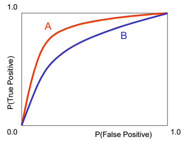

选择ROC图
傻子都知道A好。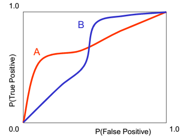 就要考虑报假警和错过病情的cost
TPr = TP/Pos = TP/(TP+FN) //有病情况下错过的概率
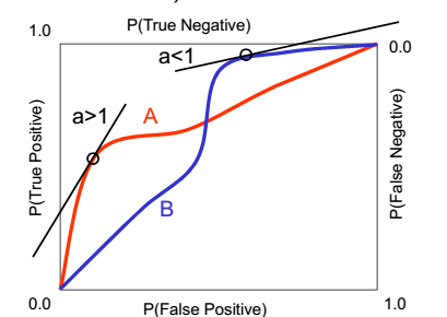 A就适合于透视,以为斜率大于1很多,保证E(N)很大的情况下FP很少;B就适合复查,不会错过病情。
Constructing ROC graphs for rating classifiers
Here is how to construct an empirical ROC for a rating classifier:1. 对training样本做一个分类估计得到估计值(估计值0-1,越高代表越pos)
2. 按估计值降序排列
3. 画出ROC 坐标,从(0,0)开始,到(Neg,Pos )也就是说每一格其实是1/Neg或1/Pos
如果该预估的真值是pos,往上画一格到(1,0)
5. 如果有一堆一样的估计值,则计数pos和neg的数量,画到长宽(neg,pos)矩形对角线
Package ‘ROCR’ for r
Descriptionperformance(prediction.obj, measure, x.measure="cutoff", ...)
measure Performance measure to use for the evaluation.
x.measure A second performance measure. If different from the default, a two-dimensional curve, withx.measure taken to be the unit in direction of the x axis, and measure to be the unit in directionof the y axis, is created. This curve is parametrized with the cutoff.
... Optional arguments (specific to individual performance measures).
ROC curves: measure="tpr", x.measure="fpr".
Precision/recall graphs: measure="prec", x.measure="rec".
Sensitivity/specificity plots: measure="sens", x.measure="spec".
Lift charts: measure="lift", x.measure="rpp".
## computing a simple ROC curve (x-axis: fpr, y-axis: tpr)
library(ROCR)
data(ROCR.simple)
pred <- prediction( ROCR.simple$predictions, ROCR.simple$labels)
perf <- performance(pred,"tpr","fpr")
plot(perf)
## precision/recall curve (x-axis: recall, y-axis: precision)
perf1 <- performance(pred, "prec", "rec")
plot(perf1)
## sensitivity/specificity curve (x-axis: specificity,y-axis: sensitivity)
perf1 <- performance(pred, "sens", "spec")
plot(perf1)
x.name: Performance measure used for the x axis.
y.name: Performance measure used for the y axis.
x.values: A list in which each entry contains the x values of the curve of this particular crossvalidation run. x.values[[i]], y.values[[i]], and alpha.values[[i]] correspond to each other.
y.values: A list in which each entry contains the y values of the curve of this particular crossvalidation run.
alpha.values: A list in which each entry contains the cutoff values of the curve of this particular cross-validation run.


 2万+
2万+

 被折叠的 条评论
为什么被折叠?
被折叠的 条评论
为什么被折叠?
 到【灌水乐园】发言


