【Python】数据分析 Section 3.4: Scales, Pivot Table | from Coursera “Applied Data Science with Python“

1. Scales

# Let's bring in pandas as normal
import pandas as pd

# Here’s an example. Lets create a dataframe of letter grades in descending order. We can also set an index
# value and here we'll just make it some human judgement of how good a student was, like "excellent" or "good"

df=pd.DataFrame(['A+', 'A', 'A-', 'B+', 'B', 'B-', 'C+', 'C', 'C-', 'D+', 'D'],
                index=['excellent', 'excellent', 'excellent', 'good', 'good', 'good', 
                       'ok', 'ok', 'ok', 'poor', 'poor'],
               columns=["Grades"])
df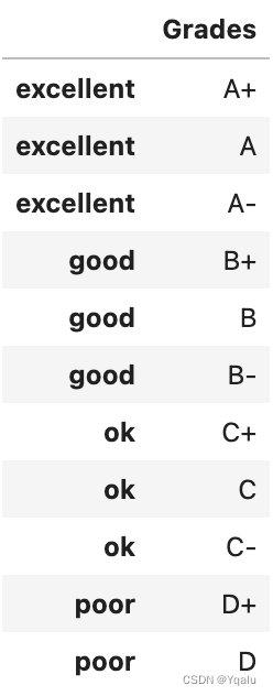

# Now, if we check the datatype of this column, we see that it's just an object, since we set string values
df.dtypes

>>> 
Grades    object
dtype: object

# We can, however, tell pandas that we want to change the type to category, using the astype() function
df["Grades"].astype("category").head()

>>> 
excellent    A+
excellent     A
excellent    A-
good         B+
good          B
Name: Grades, dtype: category
Categories (11, object): ['A', 'A+', 'A-', 'B', ..., 'C+', 'C-', 'D', 'D+']

# We see now that there are eleven categories, and pandas is aware of what those categories are. More
# interesting though is that our data isn't just categorical, but that it's ordered. That is, an A- comes
# after a B+, and B comes before a B+. We can tell pandas that the data is ordered by first creating a new
# categorical data type with the list of the categories (in order) and the ordered=True flag
my_categories=pd.CategoricalDtype(categories=['D', 'D+', 'C-', 'C', 'C+', 'B-', 'B', 'B+', 'A-', 'A', 'A+'], 
                           ordered=True)
# then we can just pass this to the astype() function
grades=df["Grades"].astype(my_categories)
grades.head()

>>>
excellent    A+
excellent     A
excellent    A-
good         B+
good          B
Name: Grades, dtype: category
Categories (11, object): ['D' < 'D+' < 'C-' < 'C' ... 'B+' < 'A-' < 'A' < 'A+']

# Now we see that pandas is not only aware that there are 11 categories, but it is also aware of the order of
# those categoreies. So, what can you do with this? Well because there is an ordering this can help with
# comparisons and boolean masking. For instance, if we have a list of our grades and we compare them to a “C”
# we see that the lexicographical comparison returns results we were not intending. 

df[df["Grades"]>"C"]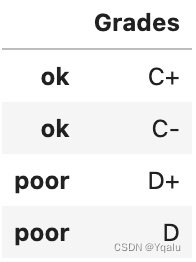

# So a C+ is great than a C, but a C- and D certainly are not. However, if we broadcast over the dataframe
# which has the type set to an ordered categorical

grades[grades>"C"]

>>> 
excellent    A+
excellent     A
excellent    A-
good         B+
good          B
good         B-
ok           C+
Name: Grades, dtype: category
Categories (11, object): ['D' < 'D+' < 'C-' < 'C' ... 'B+' < 'A-' < 'A' < 'A+']

# We see that the operator works as we would expect. We can then use a certain set of mathematical operators,
# like minimum, maximum, etc., on the ordinal data.

# Sometimes it is useful to represent categorical values as each being a column with a true or a false as to
# whether the category applies. This is especially common in feature extraction, which is a topic in the data
# mining course. Variables with a boolean value are typically called dummy variables, and pandas has a built
# in function called get_dummies which will convert the values of a single column into multiple columns of
# zeros and ones indicating the presence of the dummy variable. I rarely use it, but when I do it's very
# handy.

# There’s one more common scale-based operation I’d like to talk about, and that’s on converting a scale from
# something that is on the interval or ratio scale, like a numeric grade, into one which is categorical. Now,
# this might seem a bit counter intuitive to you, since you are losing information about the value. But it’s
# commonly done in a couple of places. For instance, if you are visualizing the frequencies of categories,
# this can be an extremely useful approach, and histograms are regularly used with converted interval or ratio
# data. In addition, if you’re using a machine learning classification approach on data, you need to be using
# categorical data, so reducing dimensionality may be useful just to apply a given technique. Pandas has a
# function called cut which takes as an argument some array-like structure like a column of a dataframe or a
# series. It also takes a number of bins to be used, and all bins are kept at equal spacing.
 
# Lets go back to our census data for an example. We saw that we could group by state, then aggregate to get a
# list of the average county size by state. If we further apply cut to this with, say, ten bins, we can see
# the states listed as categoricals using the average county size.

# let's bring in numpy
import numpy as np

# Now we read in our dataset
df=pd.read_csv("datasets/census.csv")

# And we reduce this to country data
df=df[df['SUMLEV']==50]

# And for a few groups
df=df.set_index('STNAME').groupby(level=0)['CENSUS2010POP'].agg(np.average)

df.head()

>>>
STNAME
Alabama        71339.343284
Alaska         24490.724138
Arizona       426134.466667
Arkansas       38878.906667
California    642309.586207
Name: CENSUS2010POP, dtype: float64

# Now if we just want to make "bins" of each of these, we can use cut()
pd.cut(df,10)

>>>
STNAME
Alabama                   (11706.087, 75333.413]
Alaska                    (11706.087, 75333.413]
Arizona                 (390320.176, 453317.529]
Arkansas                  (11706.087, 75333.413]
California              (579312.234, 642309.586]
Colorado                 (75333.413, 138330.766]
Connecticut             (390320.176, 453317.529]
Delaware                (264325.471, 327322.823]
District of Columbia    (579312.234, 642309.586]
Florida                 (264325.471, 327322.823]
Georgia                   (11706.087, 75333.413]
Hawaii                  (264325.471, 327322.823]
Idaho                     (11706.087, 75333.413]
Illinois                 (75333.413, 138330.766]
Indiana                   (11706.087, 75333.413]
Iowa                      (11706.087, 75333.413]
Kansas                    (11706.087, 75333.413]
Kentucky                  (11706.087, 75333.413]
Louisiana                 (11706.087, 75333.413]
Maine                    (75333.413, 138330.766]
Maryland                (201328.118, 264325.471]
Massachusetts           (453317.529, 516314.881]
Michigan                 (75333.413, 138330.766]
Minnesota                 (11706.087, 75333.413]
Mississippi               (11706.087, 75333.413]
Missouri                  (11706.087, 75333.413]
Montana                   (11706.087, 75333.413]
Nebraska                  (11706.087, 75333.413]
Nevada                  (138330.766, 201328.118]
New Hampshire            (75333.413, 138330.766]
New Jersey              (390320.176, 453317.529]
New Mexico                (11706.087, 75333.413]
New York                (264325.471, 327322.823]
North Carolina           (75333.413, 138330.766]
North Dakota              (11706.087, 75333.413]
Ohio                     (75333.413, 138330.766]
Oklahoma                  (11706.087, 75333.413]
Oregon                   (75333.413, 138330.766]
Pennsylvania            (138330.766, 201328.118]
Rhode Island            (201328.118, 264325.471]
South Carolina           (75333.413, 138330.766]
South Dakota              (11706.087, 75333.413]
Tennessee                 (11706.087, 75333.413]
Texas                    (75333.413, 138330.766]
Utah                     (75333.413, 138330.766]
Vermont                   (11706.087, 75333.413]
Virginia                  (11706.087, 75333.413]
Washington              (138330.766, 201328.118]
West Virginia             (11706.087, 75333.413]
Wisconsin                (75333.413, 138330.766]
Wyoming                   (11706.087, 75333.413]
Name: CENSUS2010POP, dtype: category
Categories (10, interval[float64, right]): [(11706.087, 75333.413] < (75333.413, 138330.766] < (138330.766, 201328.118] < (201328.118, 264325.471] ... (390320.176, 453317.529] < (453317.529, 516314.881] < (516314.881, 579312.234] < (579312.234, 642309.586]]

# Here we see that states like alabama and alaska fall into the same category, while california and the
# disctrict of columbia fall in a very different category.

# Now, cutting is just one way to build categories from your data, and there are many other methods. For
# instance, cut gives you interval data, where the spacing between each category is equal sized. But sometimes
# you want to form categories based on frequency – you want the number of items in each bin to the be the
# same, instead of the spacing between bins. It really depends on what the shape of your data is, and what
# you’re planning to do with it.

2. Pivot Tables

A pivot table is a way of summarizing data in a DataFrame for a particular purpose. It makes heavy use of the aggregation function. A pivot table is itself a DataFrame, where the rows represent one variable that you're interested in, the columns another, and the cell's some aggregate value. A pivot table also tends to includes marginal values as well, which are the sums for each column and row. This allows you to be able to see the relationship between two variables at just a glance.

# Lets take a look at pivot tables in pandas
import pandas as pd
import numpy as np

# Here we have the Times Higher Education World University Ranking dataset, which is one of the most
# influential university measures. Let's import the dataset and see what it looks like
df = pd.read_csv('datasets/cwurData.csv')
df.head()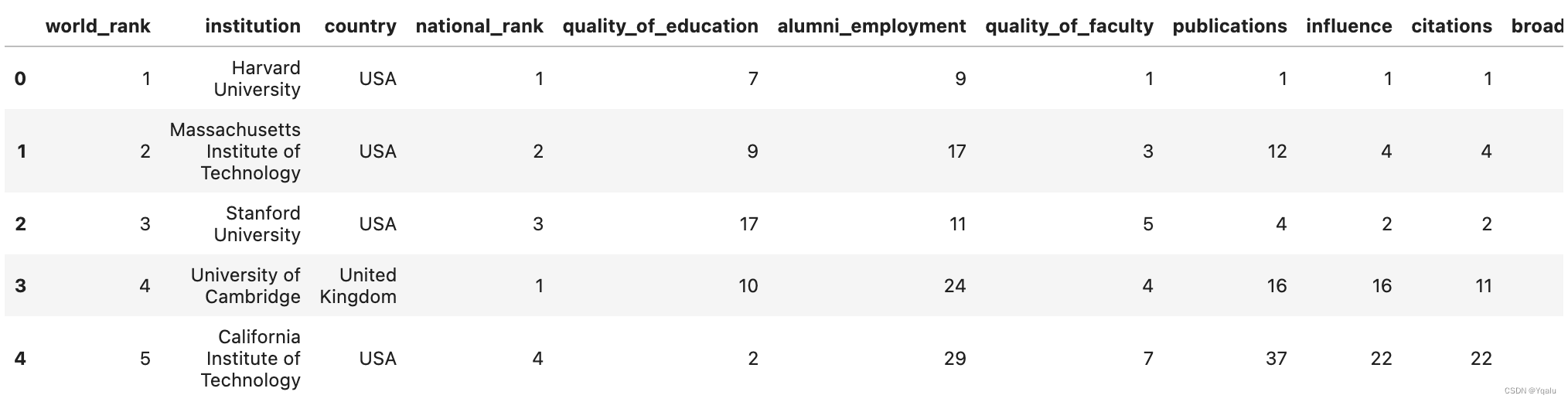

# Here we can see each institution's rank, country, quality of education, other metrics, and overall score.
# Let's say we want to create a new column called Rank_Level, where institutions with world ranking 1-100 are
# categorized as first tier and those with world ranking 101 - 200 are second tier, ranking 201 - 300 are
# third tier, after 301 is other top universities.

# Now, you actually already have enough knowledge to do this, so why don't you pause the video and give it a
# try?

# Here's my solution, I'm going to create a function called create_category which will operate on the first
# column in the dataframe, world_rank
def create_category(ranking):
    # Since the rank is just an integer, I'll just do a bunch of if/elif statements
    if (ranking >= 1) & (ranking <= 100):
        return "First Tier Top Unversity"
    elif (ranking >= 101) & (ranking <= 200):
        return "Second Tier Top Unversity"
    elif (ranking >= 201) & (ranking <= 300):
        return "Third Tier Top Unversity"
    return "Other Top Unversity"

# Now we can apply this to a single column of data to create a new series
df['Rank_Level'] = df['world_rank'].apply(lambda x: create_category(x))
# And lets look at the result
df.head()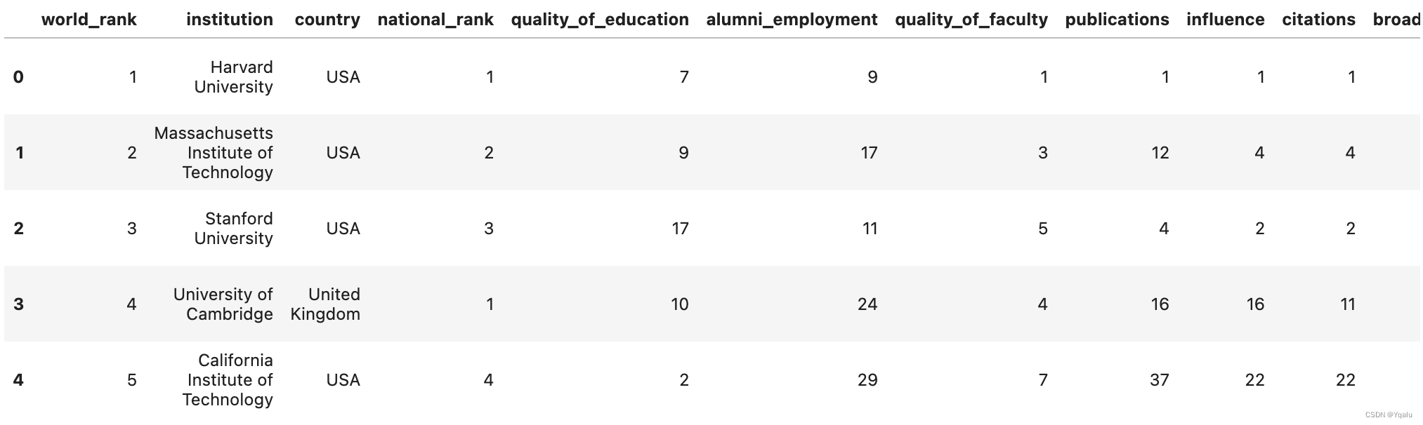

# A pivot table allows us to pivot out one of these columns a new column headers and compare it against
# another column as row indices. Let's say we want to compare rank level versus country of the universities
# and we want to compare in terms of overall score

# To do this, we tell Pandas we want the values to be Score, and index to be the country and the columns to be
# the rank levels. Then we specify that the aggregation function, and here we'll use the NumPy mean to get the
# average rating for universities in that country

df.pivot_table(values='score', index='country', columns='Rank_Level', aggfunc=[np.mean]).head()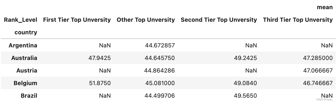

# We can see a  hierarchical dataframe where the index, or rows, are by country and the columns have two
# levels, the top level indicating that the mean value is being used and the second level being our ranks. In
# this example we only have one variable, the mean, that we are looking at, so we don't really need a
# heirarchical index.

# We notice that there are some NaN values, for example, the first row, Argentia. The NaN values indicate that
# Argentia has only observations in the "Other Top Unversities" category

# Now, pivot tables aren't limited to one function that you might want to apply. You can pass a named
# parameter, aggfunc, which is a list of the different functions to apply, and pandas will provide you with
# the result using hierarchical column names.  Let's try that same query, but pass in the max() function too

df.pivot_table(values='score', index='country', columns='Rank_Level', aggfunc=[np.mean, np.max]).head()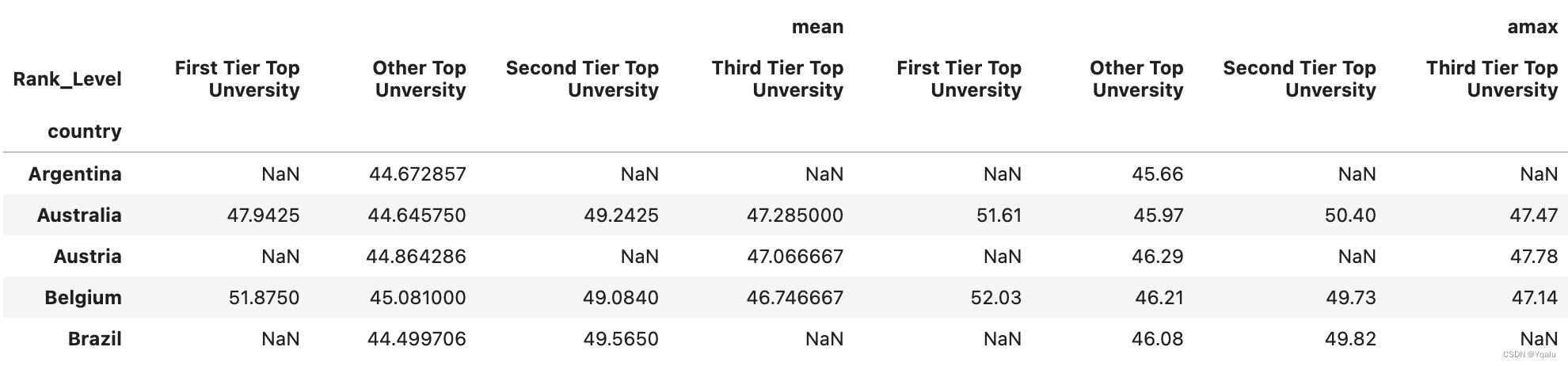

# So now we see we have both the mean and the max. As mentioned earlier, we can also summarize the values
# within a given top level column. For instance, if we want to see an overall average for the country for the
# mean and we want to see the max of the max, we can indicate that we want pandas to provide marginal values
df.pivot_table(values='score', index='country', columns='Rank_Level', aggfunc=[np.mean, np.max], 
               margins=True).head()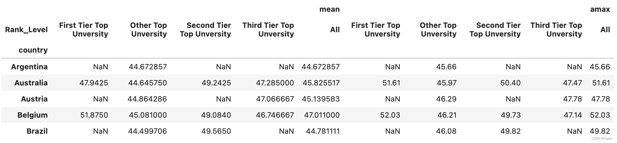

# A pivot table is just a multi-level dataframe, and we can access series or cells in the dataframe in a similar way 
# as we do so for a regular dataframe. 

# Let's create a new dataframe from our previous example
new_df=df.pivot_table(values='score', index='country', columns='Rank_Level', aggfunc=[np.mean, np.max], 
               margins=True)
# Now let's look at the index
print(new_df.index)
# And let's look at the columns
print(new_df.columns)

>>> 
Index(['Argentina', 'Australia', 'Austria', 'Belgium', 'Brazil', 'Bulgaria',
       'Canada', 'Chile', 'China', 'Colombia', 'Croatia', 'Cyprus',
       'Czech Republic', 'Denmark', 'Egypt', 'Estonia', 'Finland', 'France',
       'Germany', 'Greece', 'Hong Kong', 'Hungary', 'Iceland', 'India', 'Iran',
       'Ireland', 'Israel', 'Italy', 'Japan', 'Lebanon', 'Lithuania',
       'Malaysia', 'Mexico', 'Netherlands', 'New Zealand', 'Norway', 'Poland',
       'Portugal', 'Puerto Rico', 'Romania', 'Russia', 'Saudi Arabia',
       'Serbia', 'Singapore', 'Slovak Republic', 'Slovenia', 'South Africa',
       'South Korea', 'Spain', 'Sweden', 'Switzerland', 'Taiwan', 'Thailand',
       'Turkey', 'USA', 'Uganda', 'United Arab Emirates', 'United Kingdom',
       'Uruguay', 'All'],
      dtype='object', name='country')
MultiIndex([('mean',  'First Tier Top Unversity'),
            ('mean',       'Other Top Unversity'),
            ('mean', 'Second Tier Top Unversity'),
            ('mean',  'Third Tier Top Unversity'),
            ('mean',                       'All'),
            ('amax',  'First Tier Top Unversity'),
            ('amax',       'Other Top Unversity'),
            ('amax', 'Second Tier Top Unversity'),
            ('amax',  'Third Tier Top Unversity'),
            ('amax',                       'All')],
           names=[None, 'Rank_Level'])

# We can see the columns are hierarchical. The top level column indices have two categories: mean and max, and
# the lower level column indices have four categories, which are the four rank levels. How would we query this
# if we want to get the average scores of First Tier Top Unversity levels in each country? We would just need
# to make two dataframe projections, the first for the mean, then the second for the top tier
new_df['mean']['First Tier Top Unversity'].head()

>>>
country
Argentina        NaN
Australia    47.9425
Austria          NaN
Belgium      51.8750
Brazil           NaN
Name: First Tier Top Unversity, dtype: float64

# We can see that the output is a series object which we can confirm by printing the type. Remember that when
# you project a single column of values out of a DataFrame you get a series.
type(new_df['mean']['First Tier Top Unversity'])

>>> pandas.core.series.Series

# What if we want to find the country that has the maximum average score on First Tier Top University level?
# We can use the idxmax() function.
new_df['mean']['First Tier Top Unversity'].idxmax()

>>> 'United Kingdom'

# Now, the idxmax() function isn't special for pivot tables, it's a built in function to the Series object.
# We don't have time to go over all pandas functions and attributes, and I want to encourage you to explore
# the API to learn more deeply what is available to you.

# If you want to achieve a different shape of your pivot table, you can do so with the stack and unstack
# functions. Stacking is pivoting the lowermost column index to become the innermost row index. Unstacking is
# the inverse of stacking, pivoting the innermost row index to become the lowermost column index. An example
# will help make this clear

# Let's look at our pivot table first to refresh what it looks like
new_df.head()

# Now let's try stacking, this should move the lowermost column, so the tiers of the university rankings, to
# the inner most row
new_df=new_df.stack()
new_df.head()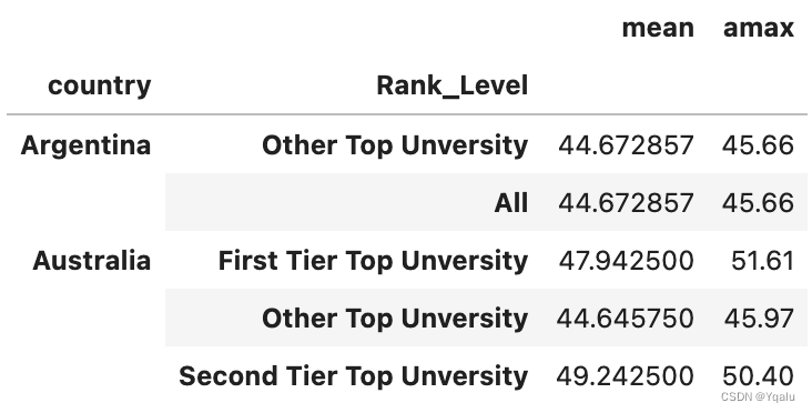

# In the original pivot table, rank levels are the lowermost column, after stacking, rank levels become the
# innermost index, appearing to the right after country

# Now let's try unstacking
new_df.unstack().head()

# That seems to restore our dataframe to its original shape. What do you think would happen if we unstacked twice in a row?
new_df.unstack().unstack().head()

>>>
      Rank_Level                country  
mean  First Tier Top Unversity  All          58.350675
                                Argentina          NaN
                                Australia    47.942500
                                Austria            NaN
                                Belgium      51.875000
dtype: float64

# We actually end up unstacking all the way to just a single column, so a series object is returned. This
# column is just a "value", the meaning of which is denoted by the heirarachical index of operation, rank, and
# country.

So that's pivot tables. This has been a pretty short description, but they're incredibly useful when dealing with numeric data, especially if you're trying to summarize the data in some form. You'll regularly be creating new pivot tables on slices of data, whether you're exploring the data yourself or preparing data for others to report on. And of course, you can pass any function you want to the aggregate function, including those that you define yourself.