


In today's lecture, where we'll be looking at the time series and date functionally in pandas. Manipulating dates and time is quite flexible in Pandas and thus allows us to conduct more analysis such as time series analysis, which we will talk about soon. Actually, pandas was originally created by Wed McKinney to handle date and time data when he worked as a consultant for hedge funds.
# Let's bring in pandas and numpy as usual
import pandas as pd
import numpy as np
1. Timestamp
# Pandas has four main time related classes. Timestamp, DatetimeIndex, Period, and PeriodIndex. First, let's
# look at Timestamp. It represents a single timestamp and associates values with points in time.

# For example, let's create a timestamp using a string 9/1/2019 10:05AM, and here we have our timestamp.
# Timestamp is interchangeable with Python's datetime in most cases.
pd.Timestamp('9/1/2019 10:05AM')

>>> Timestamp('2019-09-01 10:05:00')

# We can also create a timestamp by passing multiple parameters such as year, month, date, hour,
# minute, separately
pd.Timestamp(2019, 12, 20, 0, 0)

>>> Timestamp('2019-12-20 00:00:00')

# Timestamp also has some useful attributes, such as isoweekday(), which shows the weekday of the timestamp
# note that 1 represents Monday and 7 represents Sunday
pd.Timestamp(2019, 12, 20, 0, 0).isoweekday()

>>> 5

# You can find extract the specific year, month, day, hour, minute, second from a timestamp
pd.Timestamp(2019, 12, 20, 5, 2,23).second

>>> 23
2. Period
# Suppose we weren't interested in a specific point in time and instead wanted a span of time. This is where
# the Period class comes into play. Period represents a single time span, such as a specific day or month.

# Here we are creating a period that is January 2016,
pd.Period('1/2016')

>>> Period('2016-01', 'M')

# You'll notice when we print that out that the granularity of the period is M for month, since that was the
# finest grained piece we provided. Here's an example of a period that is March 5th, 2016.
pd.Period('3/5/2016')

>>> Period('2016-03-05', 'D')

# Period objects represent the full timespan that you specify. Arithmetic on period is very easy and
# intuitive, for instance, if we want to find out 5 months after January 2016, we simply plus 5
pd.Period('1/2016') + 5

>>> Period('2016-06', 'M')

# From the result, you can see we get June 2016. If we want to find out two days before March 5th 2016, we
# simply subtract 2
pd.Period('3/5/2016') - 2

>>> Period('2016-03-03', 'D')

# The key here is that the period object encapsulates the granularity for arithmetic
3. DatetimeIndex and PeriodIndex
# The index of a timestamp is DatetimeIndex. Let's look at a quick example. First, let's create our example
# series t1, we'll use the Timestamp of September 1st, 2nd and 3rd of 2016. When we look at the series, each
# Timestamp is the index and has a value associated with it, in this case, a, b and c.

t1 = pd.Series(list('abc'), [pd.Timestamp('2016-09-01'), pd.Timestamp('2016-09-02'),
                             pd.Timestamp('2016-09-03')])
t1

>>>
2016-09-01    a
2016-09-02    b
2016-09-03    c
dtype: object

# Looking at the type of our series index, we see that it's DatetimeIndex.
type(t1.index)

>>> pandas.core.indexes.datetimes.DatetimeIndex

# Similarly, we can create a period-based index as well.
t2 = pd.Series(list('def'), [pd.Period('2016-09'), pd.Period('2016-10'),
                             pd.Period('2016-11')])
t2

>>>
2016-09    d
2016-10    e
2016-11    f
Freq: M, dtype: object

# Looking at the type of the ts2.index, we can see that it's PeriodIndex.
type(t2.index)

>>> pandas.core.indexes.period.PeriodIndex
4. Converting to Datetime
# Now, let's look into how to convert to Datetime. Suppose we have a list of dates as strings and we want to
# create a new dataframe

# I'm going to try a bunch of different date formats
d1 = ['2 June 2013', 'Aug 29, 2014', '2015-06-26', '7/12/16']

# And just some random data
ts3 = pd.DataFrame(np.random.randint(10, 100, (4,2)), index=d1,
                   columns=list('ab'))
ts3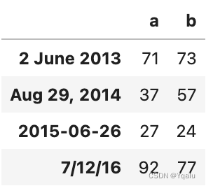
# Using pandas to_datetime, pandas will try to convert these to Datetime and put them in a standard format.

ts3.index = pd.to_datetime(ts3.index)
ts3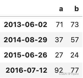
# to_datetime also() has options to change the date parse order. For example, we
# can pass in the argument dayfirst = True to parse the date in European date.

pd.to_datetime('4.7.12', dayfirst=True)

>>> Timestamp('2012-07-04 00:00:00')
4. Timedelta
# Timedeltas are differences in times. This is not the same as a a period, but conceptually similar. For
# instance, if we want to take the difference between September 3rd and  September 1st, we get a Timedelta of
# two days.
pd.Timestamp('9/3/2016')-pd.Timestamp('9/1/2016')

>>> Timedelta('2 days 00:00:00')

# We can also do something like find what the date and time is for 12 days and three hours past September 2nd,
# at 8:10 AM.
pd.Timestamp('9/2/2016 8:10AM') + pd.Timedelta('12D 3H')

>>> Timestamp('2016-09-14 11:10:00')
5. Offset
# Offset is similar to timedelta, but it follows specific calendar duration rules. Offset allows flexibility
# in terms of types of time intervals. Besides hour, day, week, month, etc it also has business day, end of
# month, semi month begin etc

# Let's create a timestamp, and see what day is that
pd.Timestamp('9/4/2016').weekday()

>>> 6

# Now we can now add the timestamp with a week ahead
pd.Timestamp('9/4/2016') + pd.offsets.Week()

>>> Timestamp('2016-09-11 00:00:00')

# Now let's try to do the month end, then we would have the last day of Septemer
pd.Timestamp('9/4/2016') + pd.offsets.MonthEnd()

>>> Timestamp('2016-09-30 00:00:00')
6. Working with Dates in a Dataframe
# Next, let's look at a few tricks for working with dates in a DataFrame. Suppose we want to look at nine
# measurements, taken bi-weekly, every Sunday, starting in October 2016. Using date_range, we can create this
# DatetimeIndex. In data_range, we have to either specify the start or end date. If it is not explicitly
# specified, by default, the date is considered the start date. Then we have to specify number of periods, and
# a frequency. Here, we set it to "2W-SUN", which means biweekly on Sunday

dates = pd.date_range('10-01-2016', periods=9, freq='2W-SUN')
dates

>>> DatetimeIndex(['2016-10-02', '2016-10-16', '2016-10-30', '2016-11-13',
               '2016-11-27', '2016-12-11', '2016-12-25', '2017-01-08',
               '2017-01-22'],
              dtype='datetime64[ns]', freq='2W-SUN')

# There are many other frequencies that you can specify. For example, you can do business day
pd.date_range('10-01-2016', periods=9, freq='B')

>>> DatetimeIndex(['2016-10-03', '2016-10-04', '2016-10-05', '2016-10-06',
               '2016-10-07', '2016-10-10', '2016-10-11', '2016-10-12',
               '2016-10-13'],
              dtype='datetime64[ns]', freq='B')

# Or you can do quarterly, with the quarter start in June
pd.date_range('04-01-2016', periods=12, freq='QS-JUN')

>>> DatetimeIndex(['2016-06-01', '2016-09-01', '2016-12-01', '2017-03-01',
               '2017-06-01', '2017-09-01', '2017-12-01', '2018-03-01',
               '2018-06-01', '2018-09-01', '2018-12-01', '2019-03-01'],
              dtype='datetime64[ns]', freq='QS-JUN')
# Now, let's go back to our weekly on Sunday example and create a DataFrame using these dates, and some random
# data, and see what we can do with it.
dates = pd.date_range('10-01-2016', periods=9, freq='2W-SUN')
df = pd.DataFrame({'Count 1': 100 + np.random.randint(-5, 10, 9).cumsum(),
'Count 2': 120 + np.random.randint(-5, 10, 9)}, index=dates)
df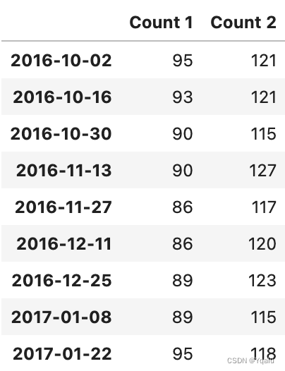
# First, we can check what day of the week a specific date is. For example, here we can see that all the dates
# in our index are on a Sunday. Which matches the frequency that we set
df.index.weekday

>>> Int64Index([6, 6, 6, 6, 6, 6, 6, 6, 6], dtype='int64')

# We can also use diff() to find the difference between each date's value.
df.diff()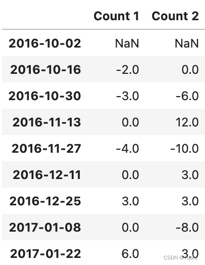
# Suppose we want to know what the mean count is for each month in our DataFrame. We can do this using
# resample. Converting from a higher frequency from a lower frequency is called downsampling (we'll talk about
# this in a moment)
df.resample('M').mean()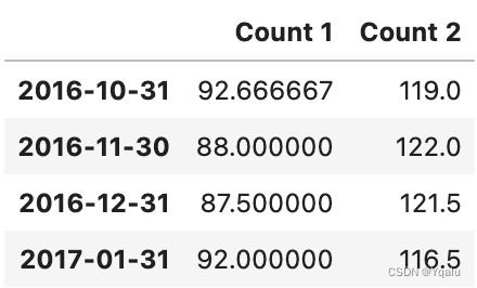
# Now let's talk about datetime indexing and slicing, which is a wonderful feature of the pandas DataFrame.
# For instance, we can use partial string indexing to find values from a particular year,
df['2017']
# Or we can do it from a particular month
df['2016-12']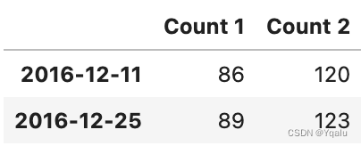
# Or we can even slice on a range of dates For example, here we only want the values from December 2016
# onwards.
df['2016-12':]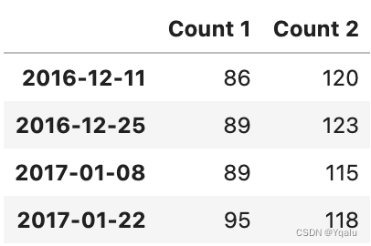
df['2016']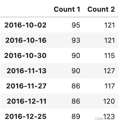


 3062
3062

 被折叠的 条评论
为什么被折叠?
被折叠的 条评论
为什么被折叠?
 到【灌水乐园】发言


