


1. DataFrame Data
The DataFrame data structure is the heart of the Panda's library. It's a primary object that you'll be working with in data analysis and cleaning tasks.
The DataFrame is conceptually a two-dimensional series object, where there's an index and multiple columns of content, with each column having a label. In fact, the distinction between a column and a row is really only a conceptual distinction. And you can think of the DataFrame itself as simply a two-axes labeled array.
1.1 create a dataframe
# Lets start by importing our pandas library
import pandas as pd

# I'm going to jump in with an example. Lets create three school records for students and their class grades. I'll create each as a series which has a student name, the class name, and the score.
record1 = pd.Series({'Name': 'Alice',
                        'Class': 'Physics',
                        'Score': 85})
record2 = pd.Series({'Name': 'Jack',
                        'Class': 'Chemistry',
                        'Score': 82})
record3 = pd.Series({'Name': 'Helen',
                        'Class': 'Biology',
                        'Score': 90})

# Like a Series, the DataFrame object is index. Here I'll use a group of series, where each series represents a row of data. Just like the Series function, we can pass in our individual items in an array, and we can pass in our index values as a second arguments
df = pd.DataFrame([record1, record2, record3],
                  index=['school1', 'school2', 'school1'])

# And just like the Series we can use the head() function to see the first several rows of the dataframe, including indices from both axes, and we can use this to verify the columns and the rows
df.head()

# You'll notice here that Jupyter creates a nice bit of HTML to render the results of the dataframe. So we have the index, which is the leftmost column and is the school name, and then we have the rows of data, where each row has a column header which was given in our initial record dictionaries

# An alternative method is that you could use a list of dictionaries, where each dictionary represents a row of data.

students = [{'Name': 'Alice',
              'Class': 'Physics',
              'Score': 85},
            {'Name': 'Jack',
             'Class': 'Chemistry',
             'Score': 82},
            {'Name': 'Helen',
             'Class': 'Biology',
             'Score': 90}]

# Then we pass this list of dictionaries into the DataFrame function
df = pd.DataFrame(students, index=['school1', 'school2', 'school1'])
# And lets print the head again
df.head()
1.2 loc & iloc
# Similar to the series, we can extract data using the .iloc and .loc attributes. Because the DataFrame is two-dimensional, passing a single value to the loc indexing operator will return the series if there's only one row to return.

# For instance, if we wanted to select data associated with school2, we would just query the .loc attribute with one parameter.
df.loc['school2']

>>>
Name          Jack
Class    Chemistry
Score           82
Name: school2, dtype: object

# You'll note that the name of the series is returned as the index value, while the column name is included in the output.

# We can check the data type of the return using the python type function.
type(df.loc['school2'])

>>> pandas.core.series.Series

# It's important to remember that the indices and column names along either axes horizontal or vertical, could be non-unique. In this example, we see two records for school1 as different rows. If we use a single value with the DataFrame lock attribute, multiple rows of the DataFrame will return, not as a new series, but as a new DataFrame.

# Lets query for school1 records
df.loc['school1']

# And we can see the the type of this is different too
type(df.loc['school1'])

>>> pandas.core.frame.DataFrame

# One of the powers of the Panda's DataFrame is that you can quickly select data based on multiple axes. For instance, if you wanted to just list the student names for school1, you would supply two parameters to .loc, one being the row index and the other being the column name.

# For instance, if we are only interested in school1's student names
df.loc['school1', 'Name']

>>>
school1    Alice
school1    Helen
Name: Name, dtype: object

# Remember, just like the Series, the pandas developers have implemented this using the indexing
# operator and not as parameters to a function.

# What would we do if we just wanted to select a single column though? Well, there are a few mechanisms. Firstly, we could transpose the matrix. This pivots all of the rows into columns and all of the columns into rows, and is done with the T attribute
df.T

# Then we can call .loc on the transpose to get the student names only
df.T.loc['Name']

>>>
school1    Alice
school2     Jack
school1    Helen
Name: Name, dtype: object

# However, since iloc and loc are used for row selection, Panda reserves the indexing operator directly on the DataFrame for column selection. In a Panda's DataFrame, columns always have a name. So this selection is always label based, and is not as confusing as it was when using the square bracket operator on the series objects. For those familiar with relational databases, this operator is analogous to column projection.
df['Name']

>>>
school1    Alice
school2     Jack
school1    Helen
Name: Name, dtype: object

# In practice, this works really well since you're often trying to add or drop new columns. However, this also means that you get a key error if you try and use .loc with a column name
df.loc['Name']

# Note too that the result of a single column projection is a Series object
type(df['Name'])

>>> pandas.core.series.Series

# Since the result of using the indexing operator is either a DataFrame or Series, you can chain operations together. For instance, we can select all of the rows which related to school1 using .loc, then project the name column from just those rows
df.loc['school1']['Name']

>>>
school1    Alice
school1    Helen
Name: Name, dtype: object

# If you get confused, use type to check the responses from resulting operations
print(type(df.loc['school1'])) #should be a DataFrame
print(type(df.loc['school1']['Name'])) #should be a Series

>>>
<class 'pandas.core.frame.DataFrame'>
<class 'pandas.core.series.Series'>

# Chaining, by indexing on the return type of another index, can come with some costs and is best avoided if you can use another approach. In particular, chaining tends to cause Pandas to return a copy of the DataFrame instead of a view on the DataFrame. For selecting data, this is not a big deal, though it might be slower than necessary. If you are changing data though this is an important distinction and can be a source of error.

# Here's another approach. As we saw, .loc does row selection, and it can take two parameters, the row index and the list of column names. The .loc attribute also supports slicing.

# If we wanted to select all rows, we can use a colon to indicate a full slice from beginning to end. This is just like slicing characters in a list in python. Then we can add the column name as the second parameter as a string. If we wanted to include multiple columns, we could do so in a list, and Pandas will bring back only the columns we have asked for.

# Here's an example, where we ask for all the names and scores for all schools using the .loc operator.
df.loc[:,['Name', 'Score']]

# Take a look at that again. The colon means that we want to get all of the rows, and the list in the second argument position is the list of columns we want to get back.
# That's selecting and projecting data from a DataFrame based on row and column labels. The key concepts to remember are that the rows and columns are really just for our benefit. Underneath this is just a two axes labeled array, and transposing the columns is easy. Also, consider the issue of chaining carefully, and try to avoid it, as it can cause unpredictable results, where your intent was to obtain a view of the data, but instead Pandas returns to you a copy.
1.3 drop
# Before we leave the discussion of accessing data in DataFrames, lets talk about dropping data.It's easy to delete data in Series and DataFrames, and we can use the drop function to do so. This function takes a single parameter, which is the index or row label, to drop. This is another tricky place for new users -- the drop function doesn't change the DataFrame by default! Instead,the drop function returns to you a copy of the DataFrame with the given rows removed.

df.drop('school1')

# But if we look at our original DataFrame we see the data is still intact.
df

# Drop has two interesting optional parameters. The first is called inplace, and if it's set to true, the DataFrame will be updated in place, instead of a copy being returned. The second parameter is the axes, which should be dropped. By default, this value is 0, indicating the row axis. But you could change it to 1 if you want to drop a column.

# For example, lets make a copy of a DataFrame using .copy()
copy_df = df.copy()
# Now lets drop the name column in this copy
copy_df.drop("Name", inplace=True, axis=1)
copy_df

# There is a second way to drop a column, and that's directly through the use of the indexing operator, using the del keyword. This way of dropping data, however, takes immediate effect on the DataFrame and does not return a view.
del copy_df['Class']
copy_df

# Finally, adding a new column to the DataFrame is as easy as assigning it to some value using the indexing operator. For instance, if we wanted to add a class ranking column with default value of None, we could do so by using the assignment operator after the square brackets.This broadcasts the default value to the new column immediately.

df['ClassRanking'] = None
df
In this lecture you've learned about the data structure you'll use the most in pandas, the DataFrame. The dataframe is indexed both by row and column, and you can easily select individual rows and project the columns you're interested in using the familiar indexing methods from the Series class. You'll be gaining a lot of experience with the DataFrame in the content to come.
2. DataFrame Indexing and Loading
In this course, we'll be largely using smaller or moderate-sized datasets. A common workflow is to read the dataset in, usually from some external file, then begin to clean and manipulate the dataset for analysis. In this lecture I'm going to demonstrate how you can load data from a comma separated file into a DataFrame.
# Lets just jump right in and talk about comma separated values (csv) files. You've undoubtedly used these -
# any spreadsheet software like excel or google sheets can save output in CSV format. It's pretty loose as a
# format, and incredibly lightweight. And totally ubiquitous.

# Now, I'm going to make a quick aside because it's convenient here. The Jupyter notebooks use ipython as the
# kernel underneath, which provides convenient ways to integrate lower level shell commands, which are
# programs run in the underlying operating system. If you're not familiar with the shell don't worry too much
# about this, but if you are, this is super handy for integration of your data science workflows. I want to
# use one shell command here called "cat", for "concatenate", which just outputs the contents of a file. In
# ipython if we prepend the line with an exclamation mark it will execute the remainder of the line as a shell
# command.  So lets look at the content of a CSV file
!cat datasets/Admission_Predict.csv

>>>
Serial No.,GRE Score,TOEFL Score,University Rating,SOP,LOR ,CGPA,Research,Chance of Admit
1,337,118,4,4.5,4.5,9.65,1,0.92
2,324,107,4,4,4.5,8.87,1,0.76
3,316,104,3,3,3.5,8,1,0.72
4,322,110,3,3.5,2.5,8.67,1,0.8
5,314,103,2,2,3,8.21,0,0.65
...

# We see from the output that there is a list of columns, and the column identifiers are listed as strings on the first line of the file. Then we have rows of data, all columns separated by commas. Now, there are lots of oddities with the CSV file format, and there is no one agreed upon specification. So you should be prepared to do a bit of work when you pull down CSV files to explore. But this lecture isn't focused on CSV files, and is more about pandas DataFrames. So lets jump into that.

# Let's bring in pandas to work with
import pandas as pd

# Pandas mades it easy to turn a CSV into a dataframe, we just call read_csv()
df = pd.read_csv('datasets/Admission_Predict.csv')

# And let's look at the first few rows
df.head()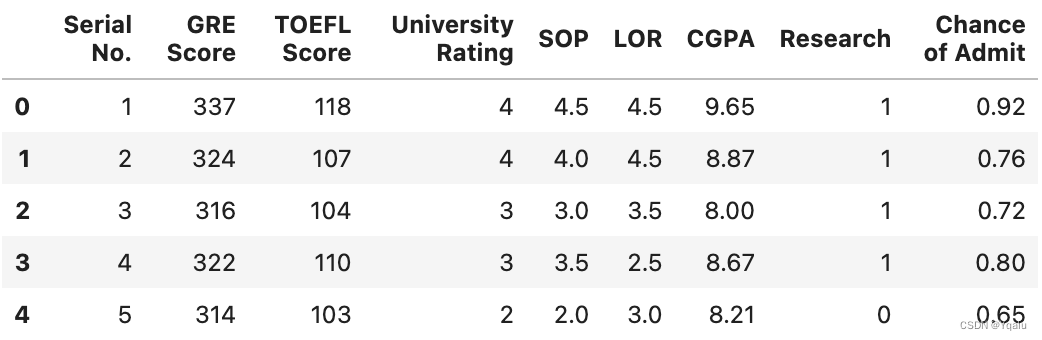
# We notice that by default index starts with 0 while the students' serial number starts from 1. If you jump back to the CSV output you'll deduce that pandas has create a new index. Instead, we can set the serial no. as the index if we want to by using the index_col.
df = pd.read_csv('datasets/Admission_Predict.csv', index_col=0)
df.head()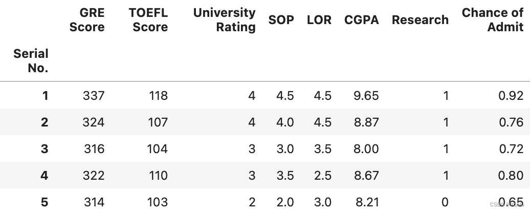
# Notice that we have two columns "SOP" and "LOR" and probably not everyone knows what they mean So let's change our column names to make it more clear. In Pandas, we can use the rename() function It takes a parameter called columns, and we need to pass into a dictionary which the keys are the old column name and the value is the corresponding new column name
new_df=df.rename(columns={'GRE Score':'GRE Score', 'TOEFL Score':'TOEFL Score',
                   'University Rating':'University Rating',
                   'SOP': 'Statement of Purpose','LOR': 'Letter of Recommendation',
                   'CGPA':'CGPA', 'Research':'Research',
                   'Chance of Admit':'Chance of Admit'})
new_df.head()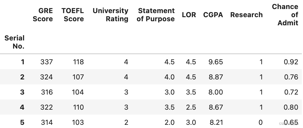
# From the output, we can see that only "SOP" is changed but not "LOR" Why is that? Let's investigate this a bit. First we need to make sure we got all the column names correct We can use the columns attribute of dataframe to get a list.
new_df.columns

>>> Index(['GRE Score', 'TOEFL Score', 'University Rating', 'Statement of Purpose',
       'LOR ', 'CGPA', 'Research', 'Chance of Admit '],
      dtype='object')

# If we look at the output closely, we can see that there is actually a space right after "LOR" and a space right after "Chance of Admit. Sneaky, huh? So this is why our rename dictionary does not work for LOR, because the key we used was just three characters, instead of "LOR "

# There are a couple of ways we could address this. One way would be to change a column by including the space in the name
new_df=new_df.rename(columns={'LOR ': 'Letter of Recommendation'})
new_df.head()
# So that works well, but it's a bit fragile. What if that was a tab instead of a space? Or two spaces? Another way is to create some function that does the cleaning and then tell renamed to apply that function across all of the data. Python comes with a handy string function to strip white space called "strip()".
# When we pass this in to rename we pass the function as the mapper parameter, and then indicate whether the axis should be columns or index (row labels)
new_df=new_df.rename(mapper=str.strip, axis='columns')
# Let's take a look at results
new_df.head()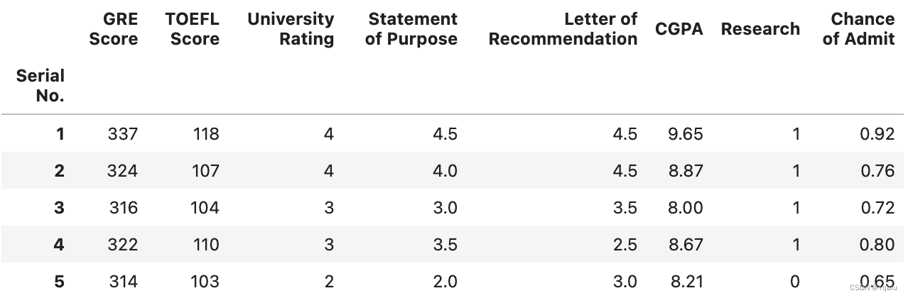
# Now we've got it - both SOP and LOR have been renamed and Chance of Admit has been trimmed up. Remember though that the rename function isn't modifying the dataframe. In this case, df is the same as it always was, there's just a copy in new_df with the changed names.
df.columns

>>> Index(['GRE Score', 'TOEFL Score', 'University Rating', 'SOP', 'LOR ', 'CGPA',
       'Research', 'Chance of Admit '],
      dtype='object')

# We can also use the df.columns attribute by assigning to it a list of column names which will directly rename the columns. This will directly modify the original dataframe and is very efficient especially when you have a lot of columns and you only want to change a few. This technique is also not affected by subtle errors in the column names, a problem that we just encountered. With a list, you can use the list index to change a certain value or use list comprehension to change all of the values

# As an example, lets change all of the column names to lower case. First we need to get our list
cols = list(df.columns)
# Then a little list comprehenshion
cols = [x.lower().strip() for x in cols]
# Then we just overwrite what is already in the .columns attribute
df.columns=cols
# And take a look at our results
df.head()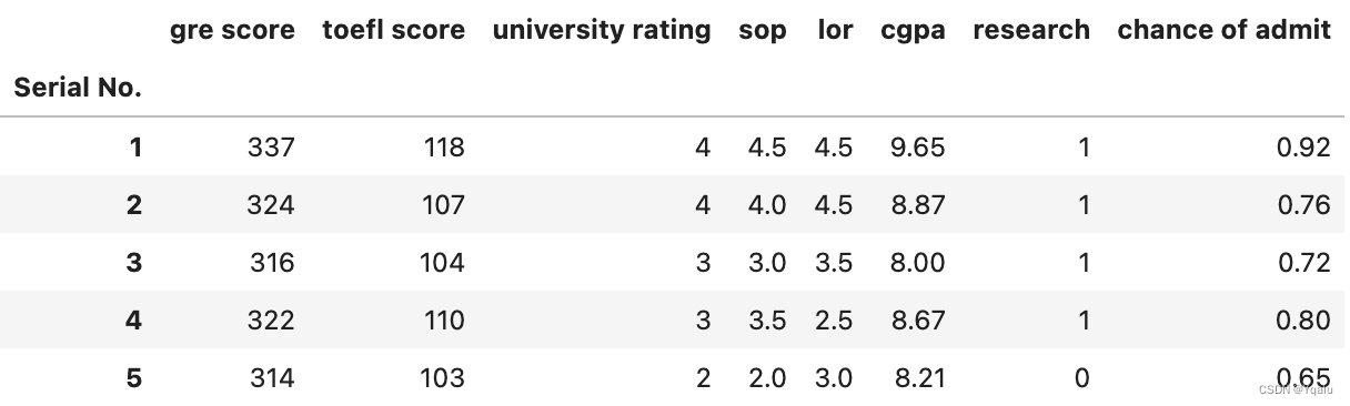
In this lecture, you've learned how to import a CSV file into a pandas DataFrame object, and how to do some basic data cleaning to the column names. The CSV file import mechanisms in pandas have lots of different options, and you really need to learn these in order to be proficient at data manipulation. Once you have set up the format and shape of a DataFrame, you have a solid start to further actions such as conducting data analysis and modeling.
Now, there are other data sources you can load directly into dataframes as well, including HTML web pages, databases, and other file formats. But the CSV is by far the most common data format you'll run into, and an important one to know how to manipulate in pandas.
3. Querying a DataFrame
In this lecture we're going to talk about querying DataFrames. The first step in the process is to understand Boolean masking. Boolean masking is the heart of fast and efficient querying in numpy and pandas, and it's analogous to bit masking used in other areas of computational science. By the end of this lecture you'll understand how Boolean masking works, and how to apply this to a DataFrame to get out data you're interested in.
A Boolean mask is an array which can be of one dimension like a series, or two dimensions like a data frame, where each of the values in the array are either true or false. This array is essentially overlaid on top of the data structure that we're querying. And any cell aligned with the true value will be admitted into our final result, and any cell aligned with a false value will not.
# Let's start with an example and import our graduate admission dataset. First we'll bring in pandas
import pandas as pd
# Then we'll load in our CSV file
df = pd.read_csv('datasets/Admission_Predict.csv', index_col=0)
# And we'll clean up a couple of poorly named columns like we did in a previous lecture
df.columns = [x.lower().strip() for x in df.columns]
# And we'll take a look at the results
df.head()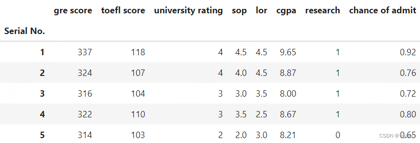
# Boolean masks are created by applying operators directly to the pandas Series or DataFrame objects.
# For instance, in our graduate admission dataset, we might be interested in seeing only those students that have a chance higher than 0.7

# To build a Boolean mask for this query, we want to project the chance of admit column using the indexing operator and apply the greater than operator with a comparison value of 0.7. This is essentially broadcasting a comparison operator, greater than, with the results being returned as a Boolean Series. The resultant Series is indexed where the value of each cell is either True or False depending on whether a student has a chance of admit higher than 0.7
admit_mask=df['chance of admit'] > 0.7
admit_mask

>>>
Serial No.
1       True
2       True
3       True
4       True
5      False
       ...
396     True
397     True
398     True
399    False
400     True
Name: chance of admit, Length: 400, dtype: bool
This is pretty fundamental, so take a moment to look at this. The result of broadcasting a comparison operator is a Boolean mask - true or false values depending upon the results of the comparison. Underneath, pandas is applying the comparison operator you specified through vectorization (so efficiently and in parallel) to all of the values in the array you specified which, in this case, is the chance of admit column of the dataframe. The result is a series, since only one column is being operator on, filled with either True or False values, which is what the comparison operator returns.
# So, what do you do with the boolean mask once you have formed it? Well, you can just lay it on top of the data to "hide" the data you don't want, which is represented by all of the False values. We do this by using the .where() function on the original DataFrame.
df.where(admit_mask).head()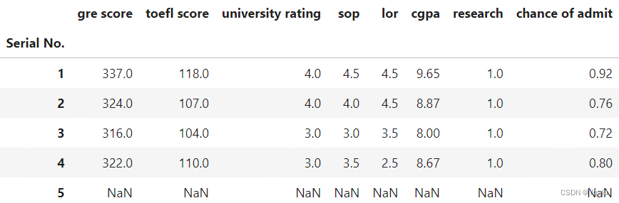
# We see that the resulting data frame keeps the original indexed values, and only data which met the condition was retained. All of the rows which did not meet the condition have NaN data instead, but these rows were not dropped from our dataset.
# The next step is, if we don't want the NaN data, we use the dropna() function
df.where(admit_mask).dropna().head()
# The returned DataFrame now has all of the NaN rows dropped. Notice the index now includes one through four and six, but not five. Despite being really handy, where() isn't actually used that often. Instead, the pandas devs created a shorthand syntax which combines where() and dropna(), doing both at once. And, in typical fashion, the just overloaded the indexing operator to do this!

df[df['chance of admit'] > 0.7].head()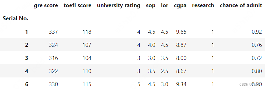
# I personally find this much harder to read, but it's also very more common when you're reading other people's code, so it's important to be able to understand it. Just reviewing this indexing operator on DataFrame, it now does two things:

# It can be called with a string parameter to project a single column
df["gre score"].head()

>>>
Serial No.
1    337
2    324
3    316
4    322
5    314
Name: gre score, dtype: int64

# Or you can send it a list of columns as strings
df[["gre score","toefl score"]].head()
# Or you can send it a boolean mask
df[df["gre score"]>320].head()
# And each of these is mimicing functionality from either .loc() or .where().dropna().

# Before we leave this, lets talk about combining multiple boolean masks, such as multiple criteria for
# including. In bitmasking in other places in computer science this is done with "and", if both masks must be
# True for a True value to be in the final mask), or "or" if only one needs to be True.

# Unfortunatly, it doesn't feel quite as natural in pandas. For instance, if you want to take two boolean
# series and and them together
(df['chance of admit'] > 0.7) and (df['chance of admit'] < 0.9)

# This doesn't work. And despite using pandas for awhile, I still find I regularly try and do this. The
# problem is that you have series objects, and python underneath doesn't know how to compare two series using
# and or or. Instead, the pandas authors have overwritten the pipe | and ampersand & operators to handle this
# for us
(df['chance of admit'] > 0.7) & (df['chance of admit'] < 0.9)

>>>
Serial No.
1      False
2       True
3       True
4       True
5      False
       ...
396     True
397     True
398    False
399    False
400    False
Name: chance of admit, Length: 400, dtype: bool

# One thing to watch out for is order of operations! A common error for new pandas users is
# to try and do boolean comparisons using the & operator but not putting parentheses around
# the individual terms you are interested in
df['chance of admit'] > 0.7 & df['chance of admit'] < 0.9

# The problem is that Python is trying to bitwise and a 0.7 and a pandas dataframe, when you really want
# to bitwise and the broadcasted dataframes together

# Another way to do this is to just get rid of the comparison operator completely, and instead
# use the built in functions which mimic this approach
df['chance of admit'].gt(0.7) & df['chance of admit'].lt(0.9)

>>>
Serial No.
1      False
2       True
3       True
4       True
5      False
       ...
396     True
397     True
398    False
399    False
400    False
Name: chance of admit, Length: 400, dtype: bool

# These functions are build right into the Series and DataFrame objects, so you can chain them
# too, which results in the same answer and the use of no visual operators. You can decide what
# looks best for you
df['chance of admit'].gt(0.7).lt(0.9)

>>>
Serial No.
1      False
2      False
3      False
4      False
5       True
       ...
396    False
397    False
398    False
399     True
400    False
Name: chance of admit, Length: 400, dtype: bool

# This only works if you operator, such as less than or greater than, is built into the DataFrame, but I certainly find that last code example much more readable than one with ampersands and parenthesis.
# You need to be able to read and write all of these, and understand the implications of the route you are choosing. It's worth really going back and rewatching this lecture to make sure you have it. I would say 50% or more of the work you'll be doing in data cleaning involves querying DataFrames.
In this lecture, we have learned to query dataframe using boolean masking, which is extremely important and often used in the world of data science. With boolean masking, we can select data based on the criteria we desire and, frankly, you'll use it everywhere. We've also seen how there are many different ways to query the DataFrame, and the interesting side implications that come up when doing so.
4. Indexing DataFrames
As we've seen, both Series and DataFrames can have indices applied to them. The index is essentially a row level label, and in pandas the rows correspond to axis zero. Indices can either be either autogenerated, such as when we create a new Series without an index, in which case we get numeric values, or they can be set explicitly, like when we use the dictionary object to create the series, or when we loaded data from the CSV file and set appropriate parameters. Another option for setting an index is to use the set_index() function. This function takes a list of columns and promotes those columns to an index. In this lecture we'll explore more about how indexes work in pandas.
# The set_index() function is a destructive process, and it doesn't keep the current index. If you want to keep the current index, you need to manually create a new column and copy into it values from the index attribute.

# Lets import pandas and our admissions dataset
import pandas as pd
df = pd.read_csv("datasets/Admission_Predict.csv", index_col=0)
df.head()
# Let's say that we don't want to index the DataFrame by serial numbers, but instead by the chance of admit. But lets assume we want to keep the serial number for later. So, lets preserve the serial number into a new column. We can do this using the indexing operator on the string that has the column label. Then we can use the set_index to set index of the column to chance of admit

# So we copy the indexed data into its own column
df['Serial Number'] = df.index
# Then we set the index to another column
df = df.set_index('Chance of Admit ')
df.head()
# You'll see that when we create a new index from an existing column the index has a name, which is the original name of the column.

# We can get rid of the index completely by calling the function reset_index(). This promotes the index into a column and creates a default numbered index.
df = df.reset_index()
df.head()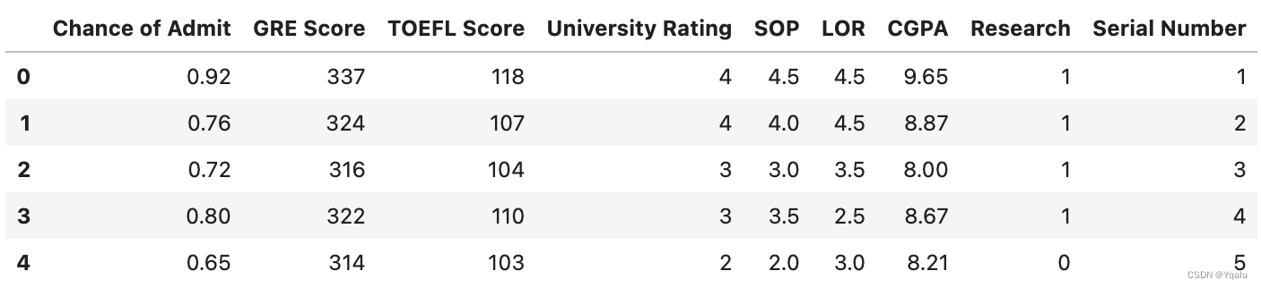
# One nice feature of Pandas is multi-level indexing. This is similar to composite keys in relational database systems. To create a multi-level index, we simply call set index and give it a list of columns that we're interested in promoting to an index.

# Pandas will search through these in order, finding the distinct data and form composite indices. A good example of this is often found when dealing with geographical data which is sorted by regions or demographics.

# Let's change data sets and look at some census data for a better example. This data is stored in the file census.csv and comes from the United States Census Bureau. In particular, this is a breakdown of the population level data at the US county level. It's a great example of how different kinds of data sets might be formatted when you're trying to clean them.

# Let's import and see what the data looks like
df = pd.read_csv('datasets/census.csv')
df.head()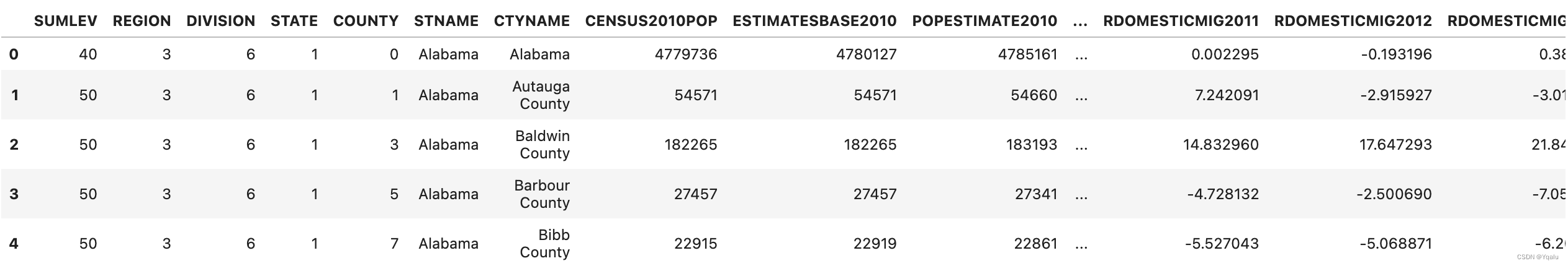
# In this data set there are two summarized levels, one that contains summary data for the whole country. And one that contains summary data for each state. I want to see a list of all the unique values in a given column. In this DataFrame, we see that the possible values for the sum level are using the unique function on the DataFrame. This is similar to the SQL distinct operator

# Here we can run unique on the sum level of our current DataFrame
df['SUMLEV'].unique()

>>> array([40, 50])

# We see that there are only two different values, 40 and 50
# Let's exclue all of the rows that are summaries at the state level and just keep the county data.
df=df[df['SUMLEV'] == 50]
df.head()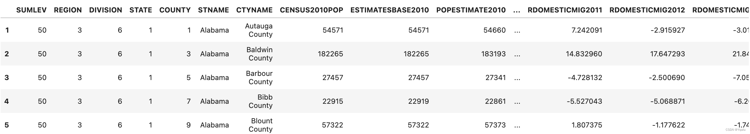
# Also while this data set is interesting for a number of different reasons, let's reduce the data that we're going to look at to just the total population estimates and the total number of births. We can do this by creating a list of column names that we want to keep then project those and assign the resulting DataFrame to our df variable.

columns_to_keep = ['STNAME','CTYNAME','BIRTHS2010','BIRTHS2011','BIRTHS2012','BIRTHS2013',
                   'BIRTHS2014','BIRTHS2015','POPESTIMATE2010','POPESTIMATE2011',
                   'POPESTIMATE2012','POPESTIMATE2013','POPESTIMATE2014','POPESTIMATE2015']
df = df[columns_to_keep]
df.head()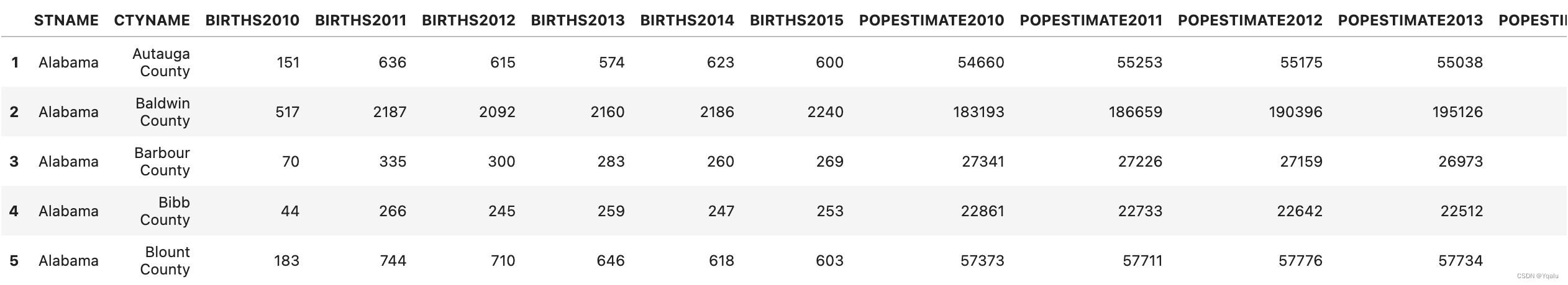
# The US Census data breaks down population estimates by state and county. We can load the data and set the index to be a combination of the state and county values and see how pandas handles it in a DataFrame. We do this by creating a list of the column identifiers we want to have indexed. And then calling set index with this list and assigning the output as appropriate. We see here that we have a dual index, first the state name and second the county name.

df = df.set_index(['STNAME', 'CTYNAME'])
df.head()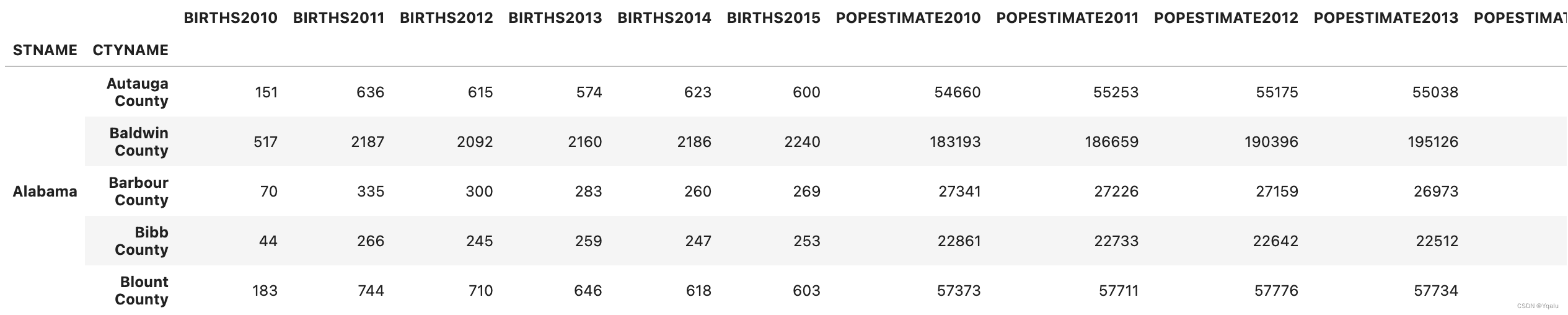
# An immediate question which comes up is how we can query this DataFrame. We saw previously that the loc attribute of the DataFrame can take multiple arguments. And it could query both the row and the columns. When you use a MultiIndex, you must provide the arguments in order by the level you wish to query. Inside of the index, each column is called a level and the outermost column is level zero.

# If we want to see the population results from Washtenaw County in Michigan the state, which is where I live, the first argument would be Michigan and the second would be Washtenaw County
df.loc['Michigan', 'Washtenaw County']

>>>
BIRTHS2010            977
BIRTHS2011           3826
BIRTHS2012           3780
BIRTHS2013           3662
BIRTHS2014           3683
BIRTHS2015           3709
POPESTIMATE2010    345563
POPESTIMATE2011    349048
POPESTIMATE2012    351213
POPESTIMATE2013    354289
POPESTIMATE2014    357029
POPESTIMATE2015    358880
Name: (Michigan, Washtenaw County), dtype: int64
# If you are interested in comparing two counties, for example, Washtenaw and Wayne County, we can pass a list of tuples describing the indices we wish to query into loc. Since we have a MultiIndex of two values, the state and the county, we need to provide two values as each element of our filtering list. Each tuple should have two elements, the first element being the first index and the second element being the second index.
# Therefore, in this case, we will have a list of two tuples, in each tuple, the first element is Michigan, and the second element is either Washtenaw County or Wayne County
df.loc[ [('Michigan', 'Washtenaw County'),
('Michigan', 'Wayne County')] ]
Okay so that's how hierarchical indices work in a nutshell. They're a special part of the pandas library which I think can make management and reasoning about data easier. Of course hierarchical labeling isn't just for rows. For example, you can transpose this matrix and now have hierarchical column labels. And projecting a single column which has these labels works exactly the way you would expect it to. Now, in reality, I don't tend to use hierarchical indicies very much, and instead just keep everything as columns and manipulate those. But, it's a unique and sophisticated aspect of pandas that is useful to know, especially if viewing your data in a tabular form.
5. Missing Values
We've seen a preview of how Pandas handles missing values using the None type and NumPy NaN values. Missing values are pretty common in data cleaning activities. And, missing values can be there for any number of reasons, and I just want to touch on a few here.
For instance, if you are running a survey and a respondant didn't answer a question the missing value is actually an omission. This kind of missing data is called Missing at Random if there are other variables that might be used to predict the variable which is missing. In my work when I delivery surveys I often find that missing data, say the interest in being involved in a follow up study, often has some correlation with another data field, like gender or ethnicity. If there is no relationship to other variables, then we call this data Missing Completely at Random (MCAR).
These are just two examples of missing data, and there are many more. For instance, data might be missing because it wasn't collected, either by the process responsible for collecting that data, such as a researcher, or because it wouldn't make sense if it were collected. This last example is extremely common when you start joining DataFrames together from multiple sources, such as joining a list of people at a university with a list of offices in the university (students generally don't have offices).
Let's look at some ways of handling missing data in pandas.
# Lets import pandas
import pandas as pd

# Pandas is pretty good at detecting missing values directly from underlying data formats, like CSV files. Although most missing valuse are often formatted as NaN, NULL, None, or N/A, sometimes missing values are not labeled so clearly. For example, I've worked with social scientists who regularly used the value of 99 in binary categories to indicate a missing value. The pandas read_csv() function has a parameter called na_values to let us specify the form of missing values. It allows scalar, string, list, or dictionaries to be used.

# Let's load a piece of data from a file called log.csv
df = pd.read_csv('datasets/class_grades.csv')
df.head(10)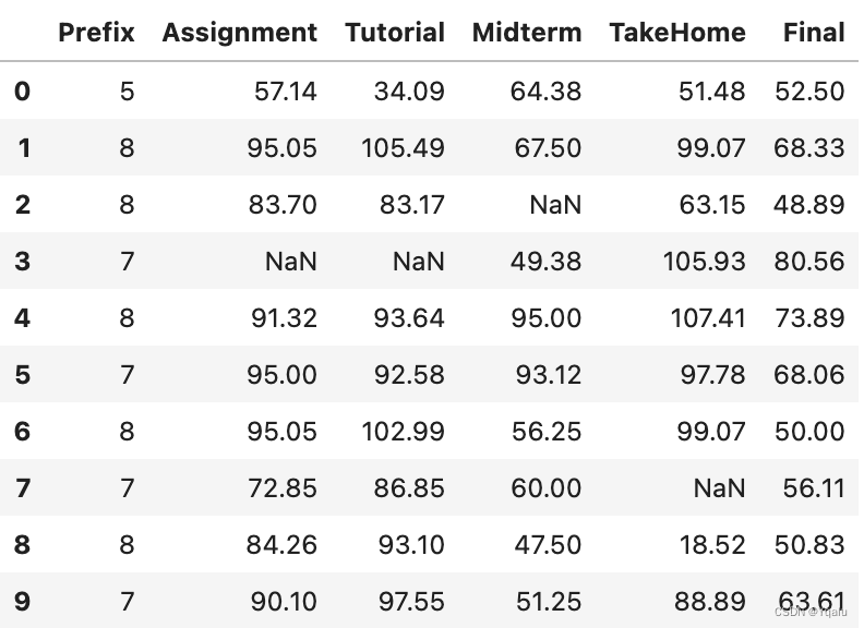
# We can actually use the function .isnull() to create a boolean mask of the whole dataframe. This effectively broadcasts the isnull() function to every cell of data.
mask=df.isnull()
mask.head(10)
# This can be useful for processing rows based on certain columns of data. Another useful operation is to be able to drop all of those rows which have any missing data, which can be done with the dropna() function.
df.dropna().head(10)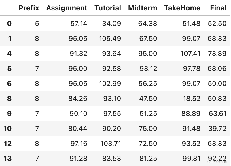
# Note how the rows indexed with 2, 3, 7, and 11 are now gone. One of the handy functions that Pandas has for working with missing values is the filling function, fillna(). This function takes a number or parameters. You could pass in a single value which is called a scalar value to change all of the missing data to one value. This isn't really applicable in this case, but it's a pretty common use case.

# So, if we wanted to fill all missing values with 0, we would use fillna
df.fillna(0, inplace=True)
df.head(10)
# Note that the inplace attribute causes pandas to fill the values inline and does not return a copy of the dataframe, but instead modifies the dataframe you have.

# We can also use the na_filter option to turn off white space filtering, if white space is an actual value of interest. But in practice, this is pretty rare. In data without any NAs, passing na_filter=False, can improve the performance of reading a large file.

# In addition to rules controlling how missing values might be loaded, it's sometimes useful to consider missing values as actually having information. I'll give an example from my own research.  I often deal with logs from online learning systems. I've looked at video use in lecture capture systems. In these systems it's common for the player for have a heartbeat functionality where playback statistics are sent to the server every so often, maybe every 30 seconds. These heartbeats can get big as they can carry the whole state of the playback system such as where the video play head is at, where the video size is, which video is being rendered to the screen, how loud the volume is.

# If we load the data file log.csv, we can see an example of what this might look like.
df = pd.read_csv("datasets/log.csv")
df.head(20)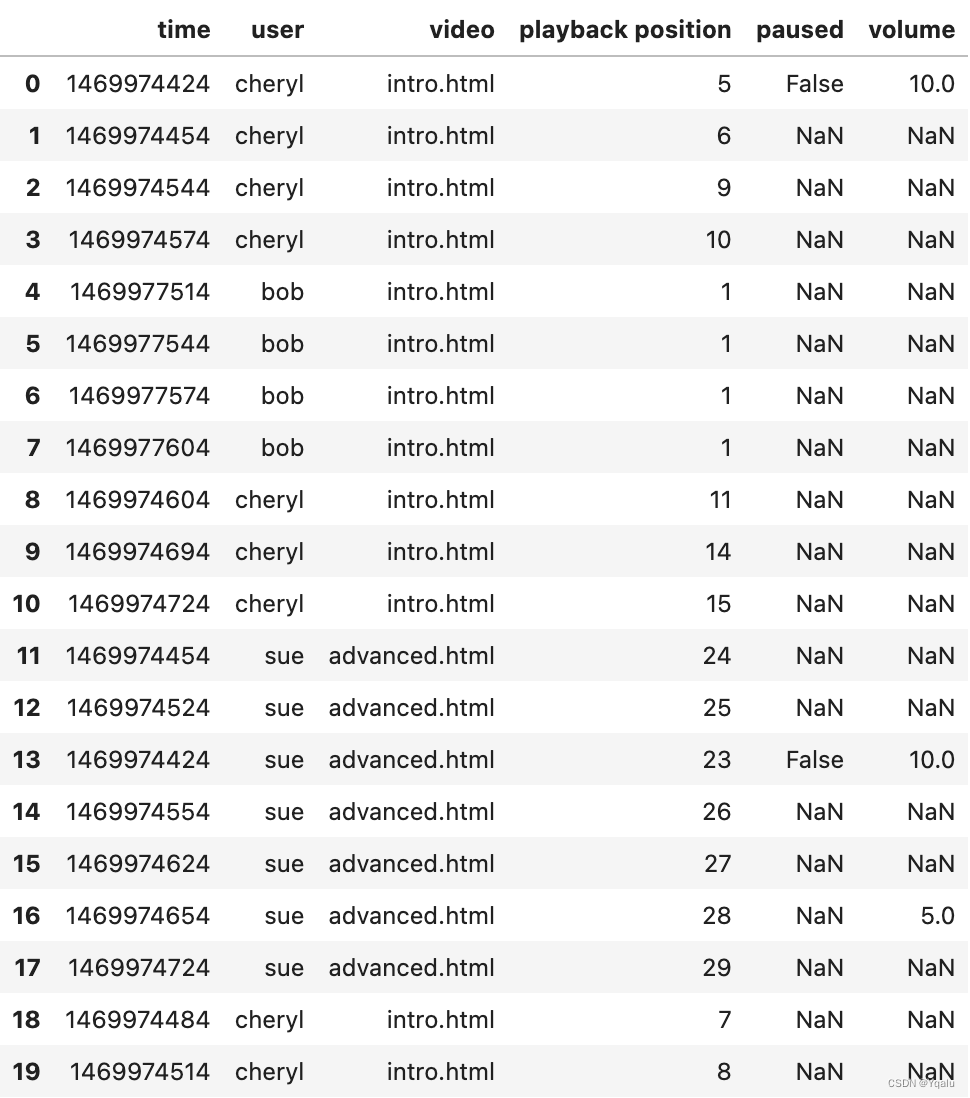
# In this data the first column is a timestamp in the Unix epoch format. The next column is the user name followed by a web page they're visiting and the video that they're playing. Each row of the DataFrame has a playback position. And we can see that as the playback position increases by one, the time stamp increases by about 30 seconds.

# Except for user Bob. It turns out that Bob has paused his playback so as time increases the playback position doesn't change. Note too how difficult it is for us to try and derive this knowledge from the data, because it's not sorted by time stamp as one might expect. This is actually not uncommon on systems which have a high degree of parallelism. There are a lot of missing values in the paused and volume columns. It's not efficient to send this information across the network if it hasn't changed. So this articular system just inserts null values into the database if there's no changes.

# Next up is the method parameter(). The two common fill values are ffill and bfill. ffill is for forward filling and it updates an na value for a particular cell with the value from the previous row. bfill is backward filling, which is the opposite of ffill. It fills the missing values with the next valid value.
# It's important to note that your data needs to be sorted in order for this to have the effect you might want. Data which comes from traditional database management systems usually has no order guarantee, just like this data. So be careful.

# In Pandas we can sort either by index or by values. Here we'll just promote the time stamp to an index then sort on the index.
df = df.set_index('time')
df = df.sort_index()
df.head(20)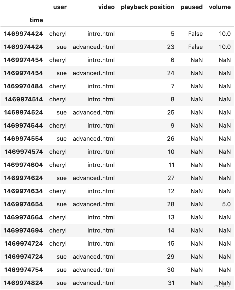
# If we look closely at the output though we'll notice that the index isn't really unique. Two users seem to be able to use the system at the same time. Again, a very common case. Let's reset the index, and use some multi-level indexing on time AND user together instead, promote the user name to a second level of the index to deal with that issue.

df = df.reset_index()
df = df.set_index(['time', 'user'])
df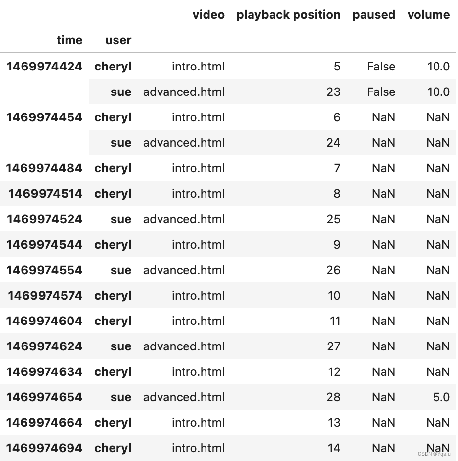
# Now that we have the data indexed and sorted appropriately, we can fill the missing datas using ffill. It's good to remember when dealing with missing values so you can deal with individual columns or sets of columns by projecting them. So you don't have to fix all missing values in one command.

df = df.fillna(method='ffill')
df.head()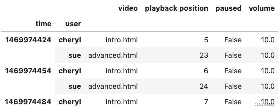
# We can also do customized fill-in to replace values with the replace() function. It allows replacement from several approaches: value-to-value, list, dictionary, regex Let's generate a simple example
df = pd.DataFrame({'A': [1, 1, 2, 3, 4],
                   'B': [3, 6, 3, 8, 9],
                   'C': ['a', 'b', 'c', 'd', 'e']})
df
# We can replace 1's with 100, let's try the value-to-value approach
df.replace(1, 100)
# How about changing two values? Let's try the list approach For example, we want to change 1's to 100 and 3's to 300
df.replace([1, 3], [100, 300])
# What's really cool about pandas replacement is that it supports regex too! Let's look at our data from the dataset logs again
df = pd.read_csv("datasets/log.csv")
df.head(20)
# To replace using a regex we make the first parameter to replace the regex pattern we want to match, the second parameter the value we want to emit upon match, and then we pass in a third parameter "regex=True".

# Take a moment to pause this video and think about this problem: imagine we want to detect all html pages in the "video" column, lets say that just means they end with ".html", and we want to overwrite that with the keyword "webpage". How could we accomplish this?

# Here's my solution, first matching any number of characters then ending in .html
df.replace(to_replace=".*.html$", value="webpage", regex=True)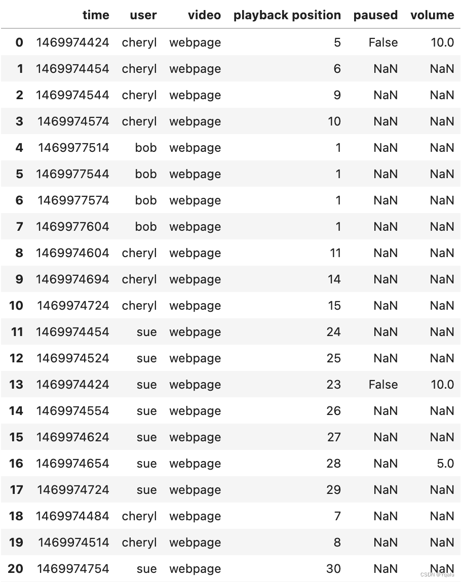
One last note on missing values. When you use statistical functions on DataFrames, these functions typically ignore missing values. For instance if you try and calculate the mean value of a DataFrame, the underlying NumPy function will ignore missing values. This is usually what you want but you should be aware that values are being excluded. Why you have missing values really matters depending upon the problem you are trying to solve. It might be unreasonable to infer missing values, for instance, if the data shouldn't exist in the first place.
6. Manipulating DataFrame
Now that you know the basics of what makes up a pandas dataframe, lets look at how we might actually clean some messy data. Now, there are many different approaches you can take to clean data, so this lecture is just one example of how you might tackle a problem.
import pandas as pd
dfs=pd.read_html("https://en.wikipedia.org/wiki/College_admissions_in_the_United_States")
len(dfs)

>>> 10

import pandas as pd
import numpy as np
import timeit

df = pd.read_csv('datasets/census.csv')
df.head()
# The first of these is called method chaining.
# The general idea behind method chaining is that every method on an object returns a reference to that object. The beauty of this is that you can condense many different operations on a DataFrame, for instance, into one line or at least one statement of code.
# Here's an example of two pieces of code in pandas using our census data.

# The first is the pandorable way to write the code with method chaining. In this code, there's no in place flag being used and you can see that when we first run a where query, then a dropna, then a set_index, and then a rename.
# You might wonder why the whole statement is enclosed in parentheses and that's just to make the statement more readable.
(df.where(df['SUMLEV']==50)
    .dropna()
    .set_index(['STNAME','CTYNAME'])
    .rename(columns={'ESTIMATESBASE2010': 'Estimates Base 2010'}))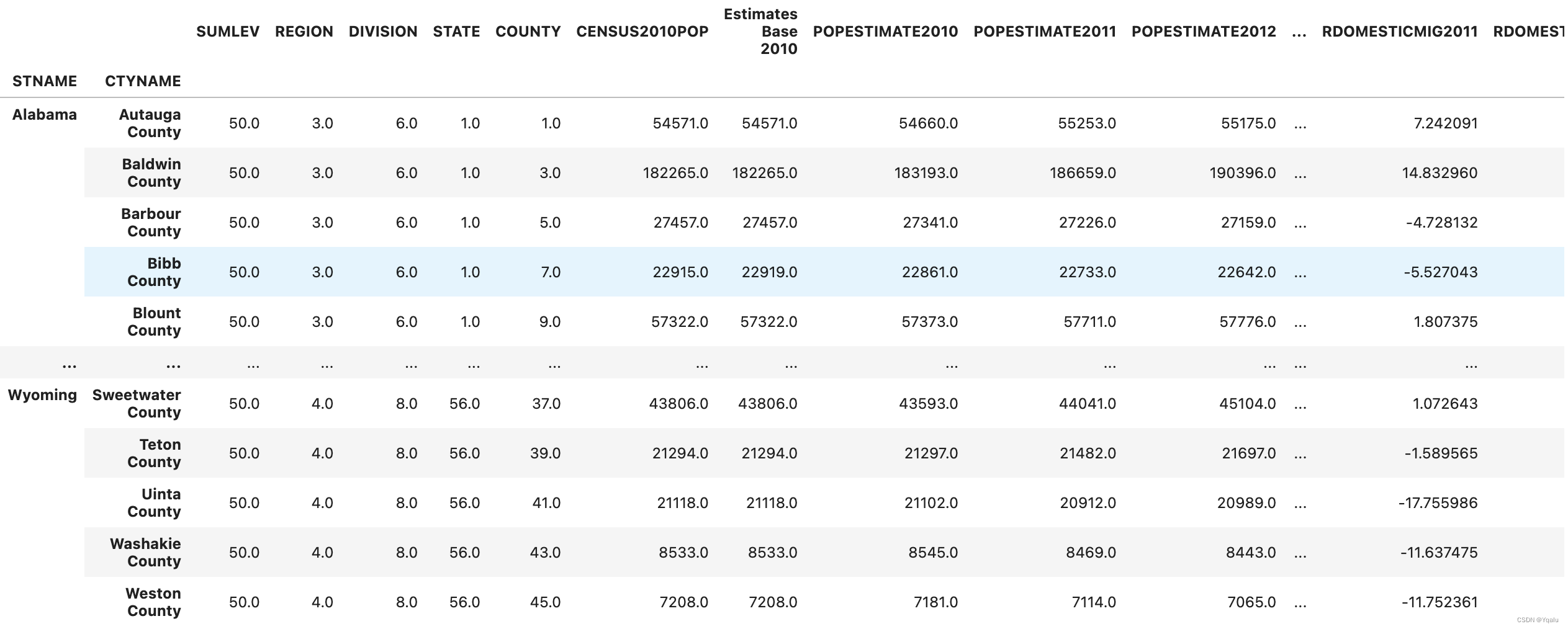
# The second example is a more traditional way of writing code.
# There's nothing wrong with this code in the functional sense, you might even be able to understand it better as a new person to the language.
# It's just not as pandorable as the first example.

df = df[df['SUMLEV']==50]
df.set_index(['STNAME','CTYNAME']).rename(columns={'ESTIMATESBASE2010': 'Estimates Base 2010'})
# Now, the key with any good idiom is to understand when it isn't helping you.
# In this case, you can actually time both methods and see which one runs faster

# We can put the approach into a function and pass the function into the timeit function to count the time the parameter number allows us to choose how many
# times we want to run the function. Here we will just set it to 1

def first_approach():
    global df
    return (df.where(df['SUMLEV']==50)
             .dropna()
             .set_index(['STNAME','CTYNAME'])
             .rename(columns={'ESTIMATESBASE2010': 'Estimates Base 2010'}))

timeit.timeit(first_approach, number=1)

>>> 0.015767341013997793

df 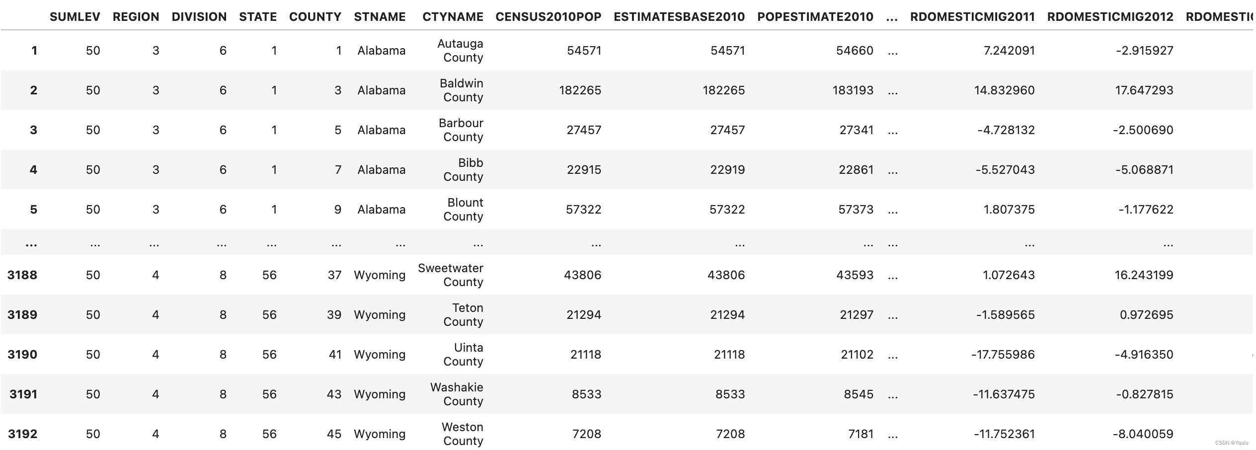
# Now let's test the second approach. As we notice, we use our global variable df in the function. However, changing a global variable inside a function will modify the variable even in a global scope and we do not want that to happen in this case. Therefore, for selecting summary levels of 50 only, I create a new dataframe for those records

# Let's run this for once and see how fast it is

def second_approach():
    global df
    new_df = df[df['SUMLEV']==50]
    new_df.set_index(['STNAME','CTYNAME'], inplace=True)
    return new_df.rename(columns={'ESTIMATESBASE2010': 'Estimates Base 2010'})
timeit.timeit(second_approach, number=1)

>>> 0.008269092999398708

# As you can see, the second approach is much faster!
# So, this is a particular example of a classic time readability trade off.

# You'll see lots of examples on stock overflow and in documentation of people
# using method chaining in their pandas. And so, I think being able to read and
# understand the syntax is really worth your time.
# Here's another pandas idiom. Python has a wonderful function called map,
# which is sort of a basis for functional programming in the language.
# When you want to use map in Python, you pass it some function you want called,
# and some iterable, like a list, that you want the function to be applied to.
# The results are that the function is called against each item in the list,
# and there's a resulting list of all of the evaluations of that function.

# Python has a similar function called applymap.
# In applymap, you provide some function which should operate on each cell of a
# DataFrame, and the return set is itself a DataFrame. Now I think applymap is
# fine, but I actually rarely use it. Instead, I find myself often wanting to
# map across all of the rows in a DataFrame. And pandas has a function that I
# use heavily there, called apply. Let's look at an example.

# Let's take our census DataFrame.
# In this DataFrame, we have five columns for population estimates.
# Each column corresponding with one year of estimates. It's quite reasonable to
# want to create some new columns for
# minimum or maximum values, and the apply function is an easy way to do this.


# First, we need to write a function which takes in a particular row of data,
# finds a minimum and maximum values, and returns a new row of data nd returns
# a new row of data.  We'll call this function min_max, this is pretty straight
# forward. We can create some small slice of a row by projecting the population
# columns. Then use the NumPy min and max functions, and create a new series
# with a label values represent the new values we want to apply.

def min_max(row):
    data = row[['POPESTIMATE2010',
                'POPESTIMATE2011',
                'POPESTIMATE2012',
                'POPESTIMATE2013',
                'POPESTIMATE2014',
                'POPESTIMATE2015']]
    return pd.Series({'min': np.min(data), 'max': np.max(data)})

# Then we just need to call apply on the DataFrame.

# Apply takes the function and the axis on which to operate as parameters.
# Now, we have to be a bit careful, we've talked about axis zero being the rows of the DataFrame in the past. But this parameter is really the parameter of the index to use. So, to apply across all rows, which is applying on all columns, you pass axis equal to one.
df.apply(min_max, axis=1)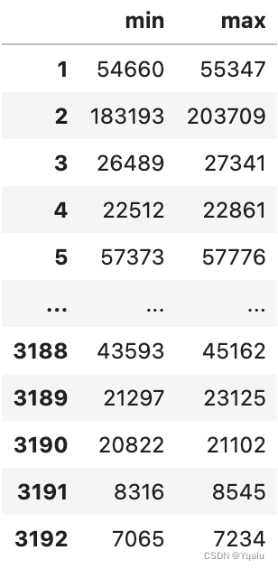
# Of course there's no need to limit yourself to returning a new series object.
# If you're doing this as part of data cleaning your likely to find yourself
# wanting to add new data to the existing DataFrame. In that case you just take
# the row values and add in new columns indicating the max and minimum scores.
# This is a regular part of my workflow when bringing in data and building
# summary or descriptive statistics.
# And is often used heavily with the merging of DataFrames.

# Here we have a revised version of the function min_max
# Instead of returning a separate series to display the min and max
# We add two new columns in the original dataframe to store min and max

def min_max(row):
    data = row[['POPESTIMATE2010',
                'POPESTIMATE2011',
                'POPESTIMATE2012',
                'POPESTIMATE2013',
                'POPESTIMATE2014',
                'POPESTIMATE2015']]
    row['max'] = np.max(data)
    row['min'] = np.min(data)
    return row
df.apply(min_max, axis=1)
# Apply is an extremely important tool in your toolkit. The reason I introduced apply here is because you rarely see it used with large function definitions, like we did. Instead, you typically see it used with lambdas. To get the most of the discussions you'll see online, you're going to need to know how to at least read lambdas.

# Here's You can imagine how you might chain several apply calls with lambdas together to create a readable yet succinct data manipulation script. One line example of how you might calculate the max of the columns using the apply function.
rows = ['POPESTIMATE2010',
        'POPESTIMATE2011',
        'POPESTIMATE2012',
        'POPESTIMATE2013',
        'POPESTIMATE2014',
        'POPESTIMATE2015']
df.apply(lambda x: np.max(x[rows]), axis=1)

>>>
1        55347
2       203709
3        27341
4        22861
5        57776
         ...
3188     45162
3189     23125
3190     21102
3191      8545
3192      7234
Length: 3142, dtype: int64

# The beauty of the apply function is that it allows flexibility in doing whatever manipulation that you desire, and the function you pass into apply can be any customized function that you write. Let's say we want to divide the states into four categories: Northeast, Midwest, South, and West
# We can write a customized function that returns the region based on the state the state regions information is obtained from Wikipedia

def get_state_region(x):
    northeast = ['Connecticut', 'Maine', 'Massachusetts', 'New Hampshire',
                 'Rhode Island','Vermont','New York','New Jersey','Pennsylvania']
    midwest = ['Illinois','Indiana','Michigan','Ohio','Wisconsin','Iowa',
               'Kansas','Minnesota','Missouri','Nebraska','North Dakota',
               'South Dakota']
    south = ['Delaware','Florida','Georgia','Maryland','North Carolina',
             'South Carolina','Virginia','District of Columbia','West Virginia',
             'Alabama','Kentucky','Mississippi','Tennessee','Arkansas',
             'Louisiana','Oklahoma','Texas']
    west = ['Arizona','Colorado','Idaho','Montana','Nevada','New Mexico','Utah',
            'Wyoming','Alaska','California','Hawaii','Oregon','Washington']

    if x in northeast:
        return "Northeast"
    elif x in midwest:
        return "Midwest"
    elif x in south:
        return "South"
    else:
        return "West"

# Now we have the customized function, let's say we want to create a new column called Region, which shows the state's region, we can use the customized function and the apply function to do so. The customized function is supposed to work on the state name column STNAME. So we will set the apply function on the state name column and pass the customized function into the apply function
df['state_region'] = df['STNAME'].apply(lambda x: get_state_region(x))

# Now let's see the results
df[['STNAME','state_region']]
So there are a couple of Pandas idioms. But I think there's many more, and I haven't talked about them here. So here's an unofficial assignment for you. Go look at some of the top ranked questions on pandas on Stack Overflow, and look at how some of the more experienced authors, answer those questions. Do you see any interesting patterns? Chime in on the course discussion forums and let's build some pandorable documents together.
7. Example
In this lecture I'm going to walk through a basic data cleaning process with you and introduce you to a few more pandas API functions.
# Let's start by bringing in pandas
import pandas as pd
# And load our dataset. We're going to be cleaning the list of presidents in the US from wikipedia
df=pd.read_csv("datasets/presidents.csv")
# And lets just take a look at some of the data
df.head()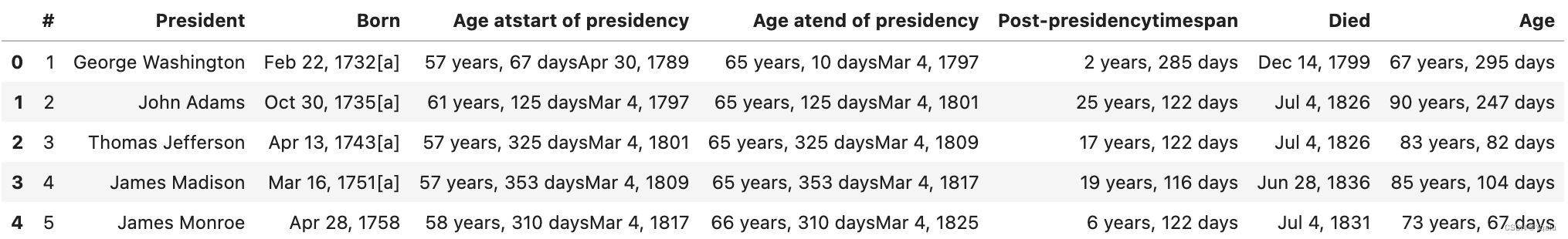
# Ok, we have some presidents, some dates, I see a bunch of footnotes in the "Born" column which might cause issues. Let's start with cleaning up that name into firstname and lastname. I'm going to tackle this with a regex. So I want to create two new columns and apply a regex to the projection of the "President" column.

# Here's one solution, we could make a copy of the President column
df["First"]=df['President']
# Then we can call replace() and just have a pattern that matches the last name and set it to an empty string
df["First"]=df["First"].replace("[ ].*", "", regex=True)
# Now let's take a look
df.head()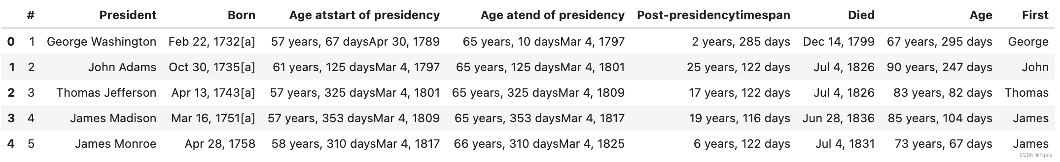
# That works, but it's kind of gross. And it's slow, since we had to make a full copy of a column then go through and update strings. There are a few other ways we can deal with this. Let me show you the most general one first, and that's called the apply() function. Let's drop the column we made first
del(df["First"])

# The apply() function on a dataframe will take some arbitrary function you have written and apply it to either a Series (a single column) or DataFrame across all rows or columns. Lets write a function which just splits a string into two pieces using a single row of data
def splitname(row):
    # The row is a single Series object which is a single row indexed by column values
    # Let's extract the firstname and create a new entry in the series
    row['First']=row['President'].split(" ")[0]
    # Let's do the same with the last word in the string
    row['Last']=row['President'].split(" ")[-1]
    # Now we just return the row and the pandas .apply() will take of merging them back into a DataFrame
    return row

# Now if we apply this to the dataframe indicating we want to apply it across columns
df=df.apply(splitname, axis='columns')
df.head()
# Pretty questionable as to whether that is less gross, but it achieves the result and I find that I use the apply() function regularly in my work. The pandas series has a couple of other nice convenience functions though, and the next I would like to touch on is called .extract(). Lets drop our firstname and lastname.
del(df['First'])
del(df['Last'])

# Extract takes a regular expression as input and specifically requires you to set capture groups that correspond to the output columns you are interested in. And, this is a great place for you to pause the video and reflect - if you were going to write a regular expression that returned groups and just had the firstname and lastname in it, what would that look like?

# Here's my solution, where we match three groups but only return two, the first and the last name
pattern="(^[\w]*)(?:.* )([\w]*$)"

# Now the extract function is built into the str attribute of the Series object, so we can call it using Series.str.extract(pattern)
df["President"].str.extract(pattern).head()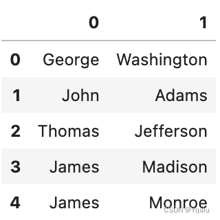
# So that looks pretty nice, other than the column names. But if we name the groups we get named columns out
pattern="(?P<First>^[\w]*)(?:.* )(?P<Last>[\w]*$)"

# Now call extract
names=df["President"].str.extract(pattern).head()
names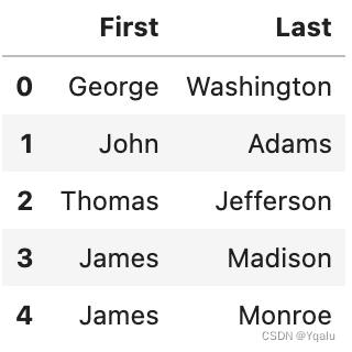
# And we can just copy these into our main dataframe if we want to
df["First"]=names["First"]
df["Last"]=names["Last"]
df.head()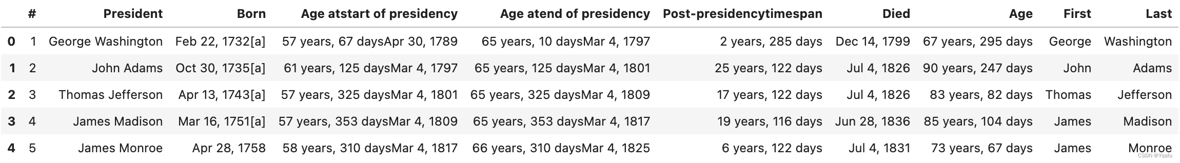
# It's worth looking at the pandas str module for other functions which have been written specifically to clean up strings in DataFrames, and you can find that in the docs in the Working with Text section: https://pandas.pydata.org/pandas-docs/stable/user_guide/text.html

# Now lets move on to clean up that Born column. First, let's get rid of anything that isn't in the pattern of Month Day and Year.
df["Born"]=df["Born"].str.extract("([\w]{3} [\w]{1,2}, [\w]{4})")
df["Born"].head()

>>>
0    Feb 22, 1732
1    Oct 30, 1735
2    Apr 13, 1743
3    Mar 16, 1751
4    Apr 28, 1758
Name: Born, dtype: object

# So, that cleans up the date format. But I'm going to foreshadow something else here - the type of this column is object, and we know that's what pandas uses when it is dealing with string. But pandas actually has really interesting date/time features - in fact, that's one of the reasons Wes McKinney put his efforts into the library, to deal with financial transactions. So if I were building this out, I would actually update this column to the write data type as well
df["Born"]=pd.to_datetime(df["Born"])
df["Born"].head()

>>>
0   1732-02-22
1   1735-10-30
2   1743-04-13
3   1751-03-16
4   1758-04-28
Name: Born, dtype: datetime64[ns]

# This would make subsequent processing on the dataframe around dates, such as getting every President who was born in a given time span, much easier.
Now, most of the other columns in this dataset I would clean in a similar fashion. And this would be a good practice activity for you, so I would recommend that you pause the video, open up the notebook for the lecture if you don't already have it opened, and then finish cleaning up this dataframe. In this lecture I introduced you to the str module which has a number of important functions for cleaning pandas dataframes. You don't have to use these - I actually use apply() quite a bit myself, especially if I don't need high performance data cleaning because my dataset is small. But the str functions are incredibly useful and build on your existing knowledge of regular expressions, and because they are vectorized they are efficient to use as well.


 被折叠的 条评论
为什么被折叠?
被折叠的 条评论
为什么被折叠?
 到【灌水乐园】发言


