


Reference:
[1]http://blog.csdn.net/richard2357/article/details/18145631
[2]http://ufldl.stanford.edu/wiki/index.php/Exercise:PCA_and_Whitening
[3]http://ufldl.stanford.edu/tutorial/unsupervised/PCAWhitening/
PCA主要就是实现降维的目的,每一个维度有均值和方差,首先可以根据协方差矩阵来判断出来哪个方向方差最大,PCA主要作用就是变换一组基。
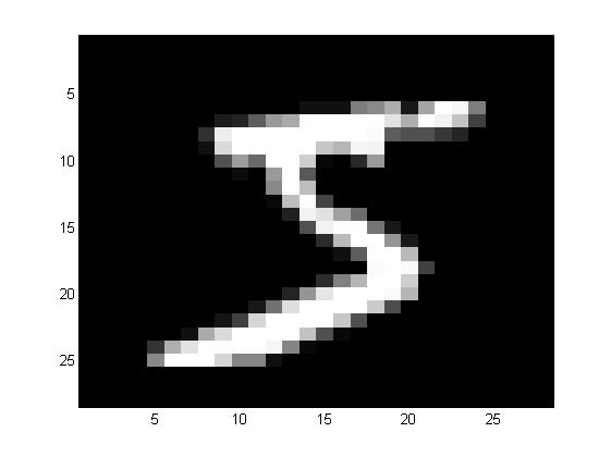
可以看一下pca之后的图片:
由于matlab是列是主,所以可以看出,经过pca之后的图,在最左边的一列是有很大变化的。所以,其实变换之后的主要信息是存储在U这个矩阵中了。
k个基的作用就是在降维的过程中去掉冗余的元素。
白化的作用就是映射之后使得其标准差为1.
ZCA的作用就是标准化之后再回来。
那么为什么ZCA就能够使得边缘增强呢?
其实ZCA相比于最传统的PCA的作用其实中间经过了标准化,标准化就降低了
1.meanmap
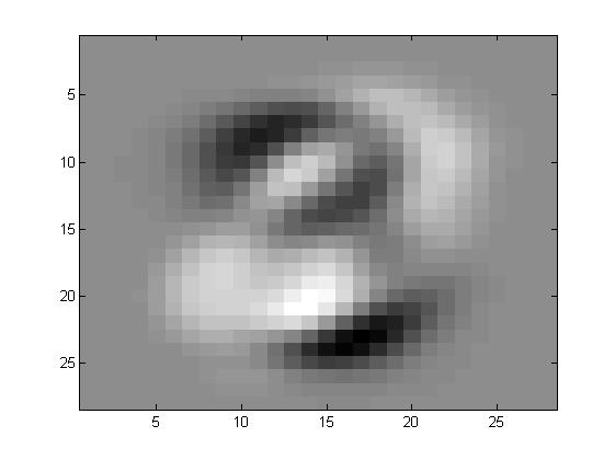
mean的作用其实就是去掉均值,可以看出来,其实有时候因为整体偏明亮或者偏暗,对于去掉之后的整体效果也会有影响。
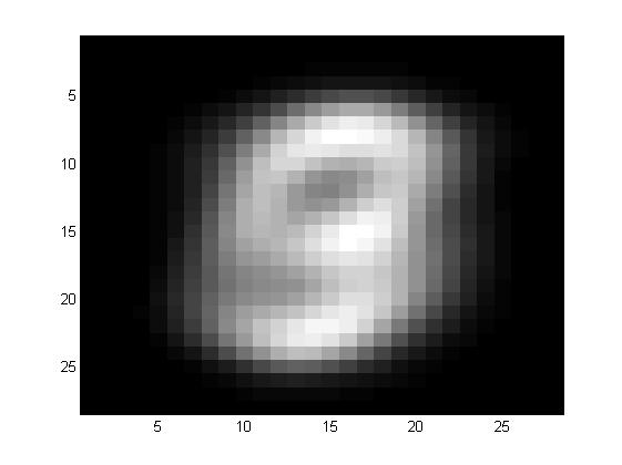
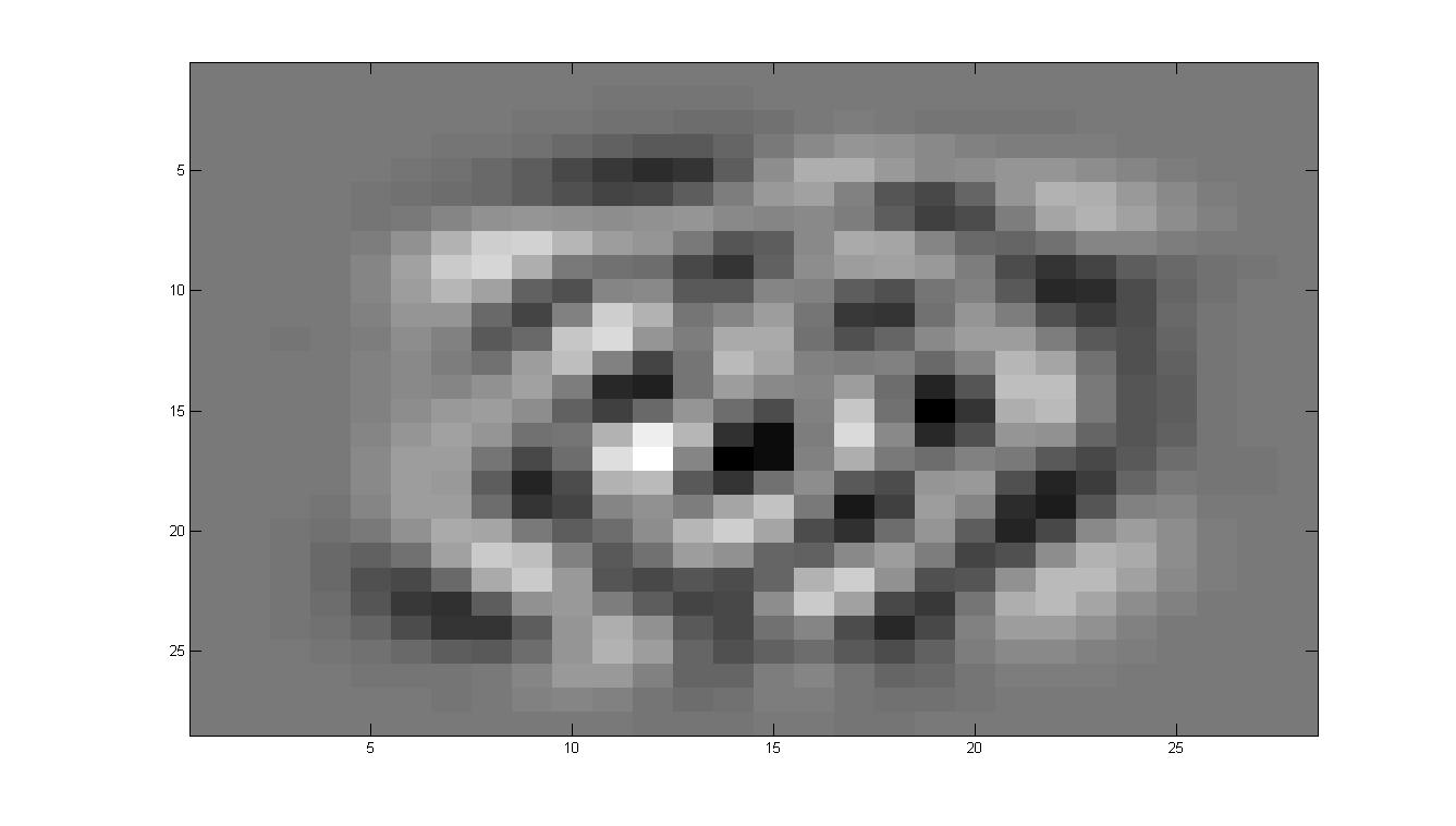
2.ZCA
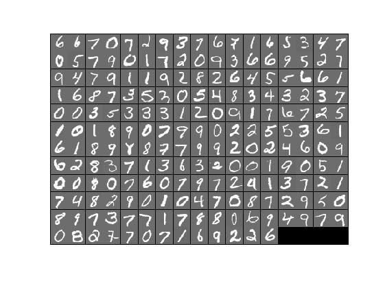
首先先来看看原始图片和ZCA之后的图片。
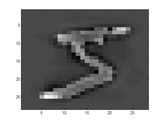
可以发现,相对于原始图片,ZCA相对来说模糊一些。
看看特征向量都是什么样子的
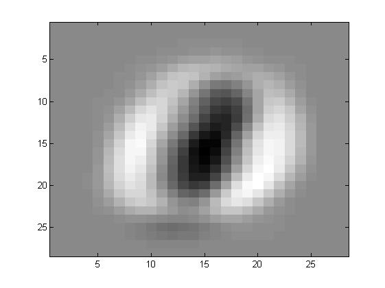
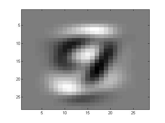
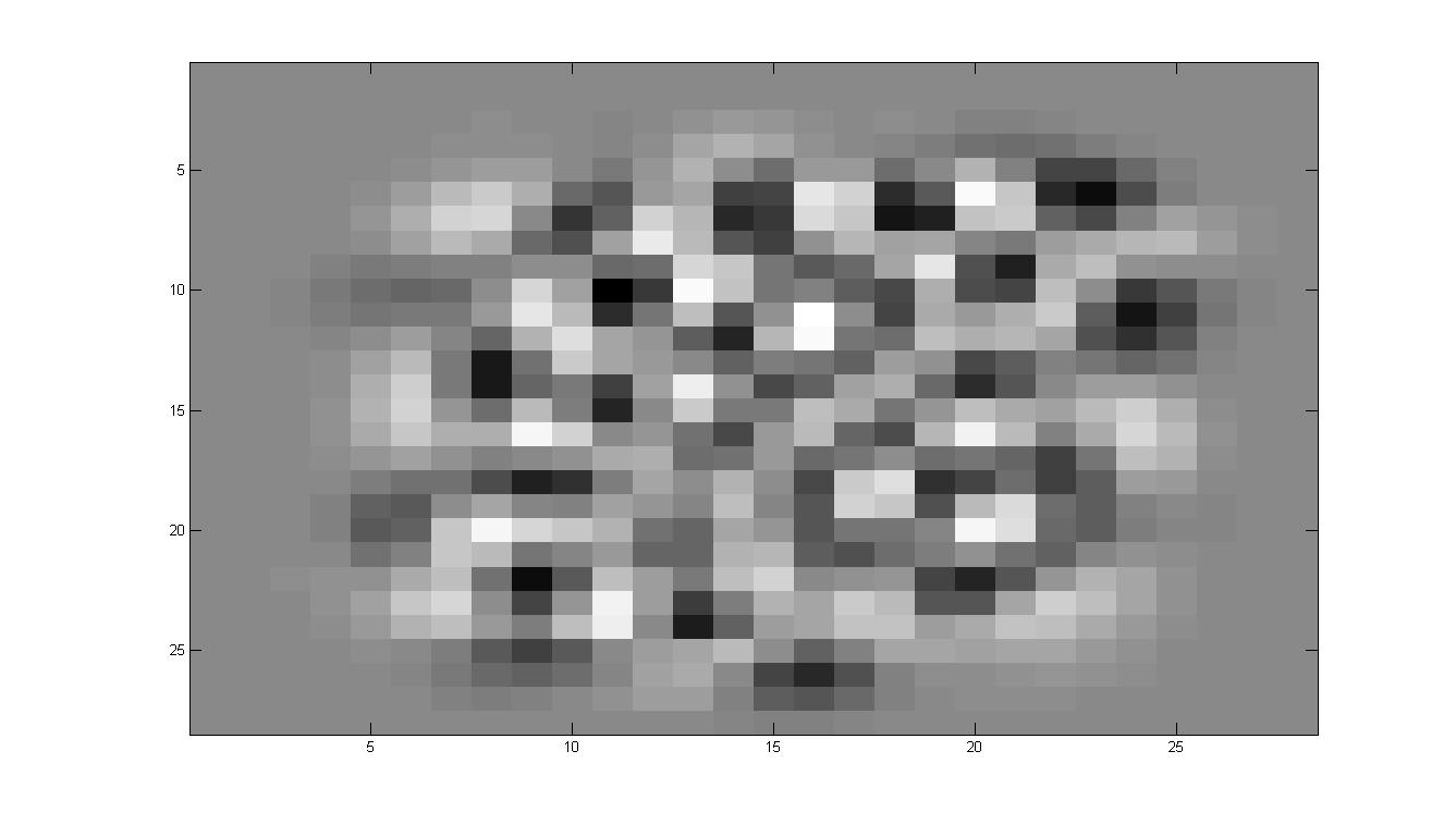
其实特征向量在前面可以发现主要的功能就是提取一些方差比较大的,什么意思呢?
比如说有一大片区域,一个数字会是1,另一个数字会是0,那么在这些向量的共同方向,注意是共同方向上,差别很大。所以最开始的特征都是有一定形状的,也就是这些部分的合方向的向量方差很大。
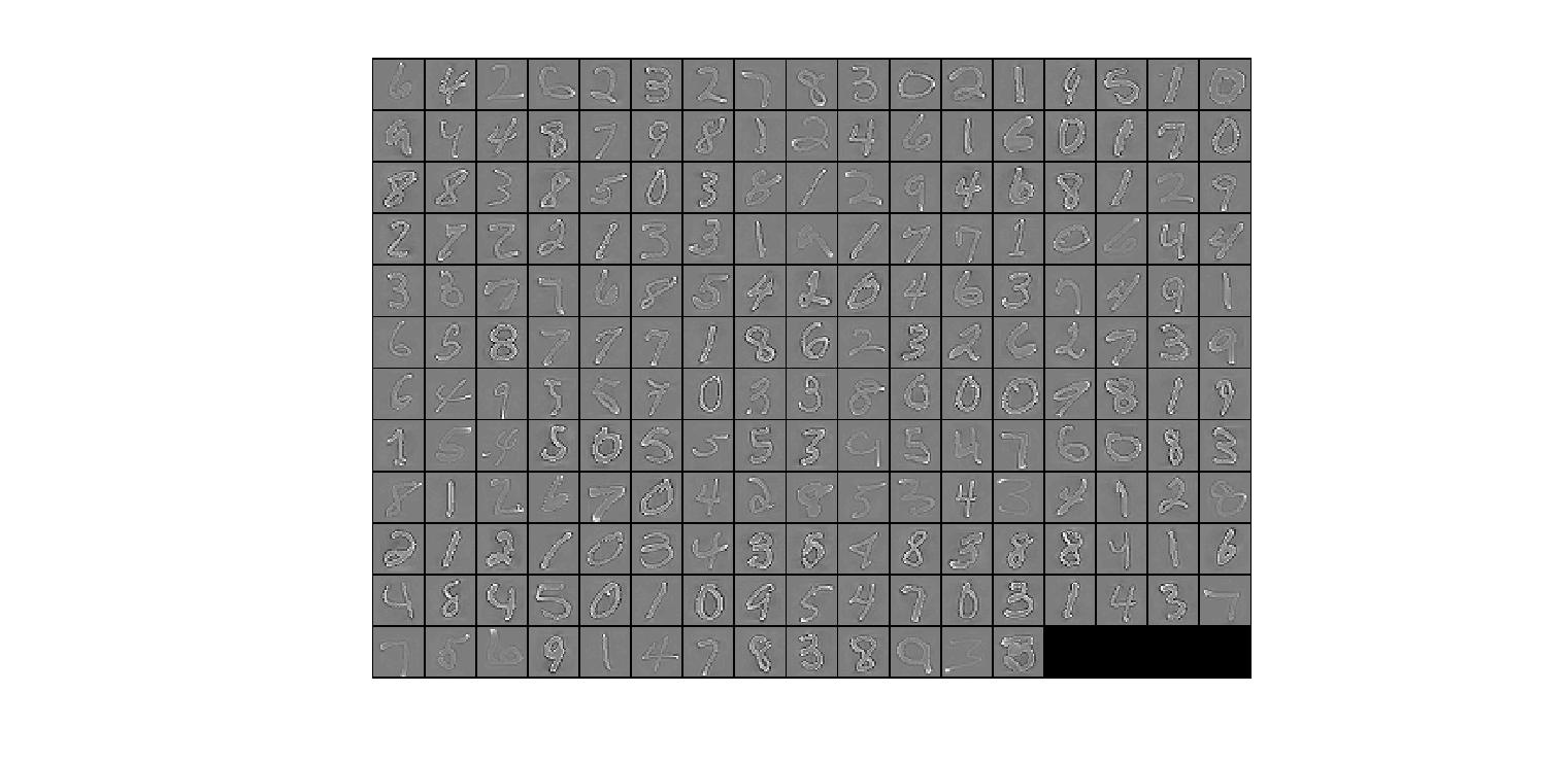
在ZCA的过程中,有一步就是白化,其作用就是削弱这些变化非常大的区域的差别,也就意味着在运行白化的过程中,那些数字之间差别非常大的区域都被相当程度的削弱,所以数字会变的区分性弱一些。而边缘因为其实并不会有着很大的影响,或者说数字之间的差别并不能形成多大的影响力,所以我们看到的效果就是,数字整体上来说,会更相似,但是边缘因为其并不具有很明显的区分性,所以会幸存下来。
从削弱作用的角度来说,epsilon越大,那么削弱作用也就越大,意味着贫富差距也就被影响的越大,就好象每个人的资产都要被稀释,但是不是按照比例来的,而是加上了一个常数,所以不是等比例的,而epsilon越小,那么就是按照比例来的,求conv之后就是一条红线。
%%================================================================
%% Step 0a: Load data
% Here we provide the code to load natural image data into x.
% x will be a 784 * 600000 matrix, where the kth column x(:, k) corresponds to
% the raw image data from the kth 12x12 image patch sampled.
% You do not need to change the code below.
addpath(genpath('../common'))
x = loadMNISTImages('../common/train-images-idx3-ubyte');
figure('name','Raw images');
randsel = randi(size(x,2),200,1); % A random selection of samples for visualization
display_network(x(:,randsel));
%%================================================================
%% Step 0b: Zero-mean the data (by row)
% You can make use of the mean and repmat/bsxfun functions.
%%% YOUR CODE HERE %%%
meanmap = mean(x,1);
x = bsxfun(@minus,x,meanmap);
%%================================================================
%% Step 1a: Implement PCA to obtain xRot
% Implement PCA to obtain xRot, the matrix in which the data is expressed
% with respect to the eigenbasis of sigma, which is the matrix U.
%%% YOUR CODE HERE %%%
sigma = x*x'/size(x,2);
[U,S,Vt] = svd(sigma);
%%================================================================
%% Step 1b: Check your implementation of PCA
% The covariance matrix for the data expressed with respect to the basis U
% should be a diagonal matrix with non-zero entries only along the main
% diagonal. We will verify this here.
% Write code to compute the covariance matrix, covar.
% When visualised as an image, you should see a straight line across the
% diagonal (non-zero entries) against a blue background (zero entries).
%%% YOUR CODE HERE %%%
y = U'*x;
covar = y*y';
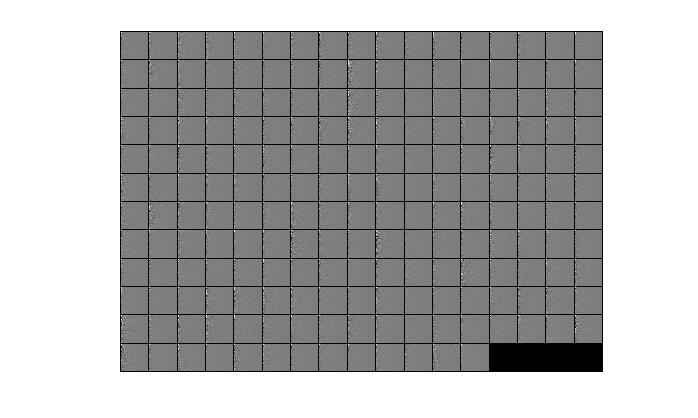
% Visualise the covariance matrix. You should see a line across the
% diagonal against a blue background.
figure('name','Visualisation of covariance matrix');
imagesc(covar);
%%================================================================
%% Step 2: Find k, the number of components to retain
% Write code to determine k, the number of components to retain in order
% to retain at least 99% of the variance.
%%% YOUR CODE HERE %%%
tmp = S(sub2ind(size(S),1:size(S,1),1:size(S,1)));
tmp = tmp ./ sum(tmp);
for i = 1:length(tmp)
if sum(tmp(1:i)) >=0.99
k = i;
break;
end
end
%%================================================================
%% Step 3: Implement PCA with dimension reduction
% Now that you have found k, you can reduce the dimension of the data by
% discarding the remaining dimensions. In this way, you can represent the
% data in k dimensions instead of the original 144, which will save you
% computational time when running learning algorithms on the reduced
% representation.
%
% Following the dimension reduction, invert the PCA transformation to produce
% the matrix xHat, the dimension-reduced data with respect to the original basis.
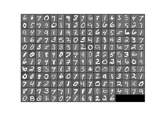
% Visualise the data and compare it to the raw data. You will observe that
% there is little loss due to throwing away the principal components that
% correspond to dimensions with low variation.
%%% YOUR CODE HERE %%%
xHat = U(:,1:k) * U(:,1:k)' * x;
% Visualise the data, and compare it to the raw data
% You should observe that the raw and processed data are of comparable quality.
% For comparison, you may wish to generate a PCA reduced image which
% retains only 90% of the variance.
figure('name',['PCA processed images ',sprintf('(%d / %d dimensions)', k, size(x, 1)),'']);
display_network(xHat(:,randsel));
figure('name','Raw images');
display_network(x(:,randsel));
%%================================================================
%% Step 4a: Implement PCA with whitening and regularisation
% Implement PCA with whitening and regularisation to produce the matrix
% xPCAWhite.
epsilon = 1e-1;
%%% YOUR CODE HERE %%%
tmp = sqrt(diag(S)+epsilon);
xPCAwhite = U' * x ./ repmat(tmp,1,size(x,2));
%% Step 4b: Check your implementation of PCA whitening
% Check your implementation of PCA whitening with and without regularisation.
% PCA whitening without regularisation results a covariance matrix
% that is equal to the identity matrix. PCA whitening with regularisation
% results in a covariance matrix with diagonal entries starting close to
% 1 and gradually becoming smaller. We will verify these properties here.
% Write code to compute the covariance matrix, covar.
%
% Without regularisation (set epsilon to 0 or close to 0),
% when visualised as an image, you should see a red line across the
% diagonal (one entries) against a blue background (zero entries).
% With regularisation, you should see a red line that slowly turns
% blue across the diagonal, corresponding to the one entries slowly
% becoming smaller.
%%% YOUR CODE HERE %%%
covar = xPCAwhite * xPCAwhite' ./ size(xPCAwhite,2);
% Visualise the covariance matrix. You should see a red line across the
% diagonal against a blue background.
figure('name','Visualisation of covariance matrix');
imagesc(covar);
%%================================================================
%% Step 5: Implement ZCA whitening
% Now implement ZCA whitening to produce the matrix xZCAWhite.
% Visualise the data and compare it to the raw data. You should observe
% that whitening results in, among other things, enhanced edges.
%%% YOUR CODE HERE %%%
xZCAWhite = U * xPCAwhite;
% Visualise the data, and compare it to the raw data.
% You should observe that the whitened images have enhanced edges.
figure('name','ZCA whitened images');
display_network(xZCAWhite(:,randsel));
figure('name','Raw images');
display_network(x(:,randsel));


 2万+
2万+

 被折叠的 条评论
为什么被折叠?
被折叠的 条评论
为什么被折叠?
 到【灌水乐园】发言


