


From Wiki
Quasi-Newton methods are methods used to either find zeroes or local maxima and minima of functions. They are an alternative to Newton's method when the Jacobian (when searching for zeroes) or the Hessian (when searching for extrema) is unavailable or too expensive to compute at every iteration.
Search for zeros
Newton's method to find zeroes of a function  of multiple variables is given by:
 ![x_{n+1} = x_n -[J_g(x_n)]^{-1} g(x_n)\,\!](http://upload.wikimedia.org/math/4/b/3/4b3df6dc8e01c48485589f81da742027.png) where
where  is the Jacobian matrix of evaluated for
  .
.
Strictly, any method that replaces the exact Jacobian with an approximation is a quasi-Newton method. The chord method (where is replaced by  for all iterations) for instance is a simple example. The methods given below for optimisation are other examples. Using methods developed to find extrema in order to find zeroes is not always a good idea as the majority of the methods used to find extrema require that the matrix that is used is symmetrical. While this holds in the context of the search for extrema, it rarely holds when searching for zeroes. Broyden's "good" method and Broyden's "bad" method are two methods commonly used to find extrema that can also be applied to find zeroes. Other methods that can be used are the Column Updating Method, the Inverse Column Updating Method, the Quasi-Newton Least Squares Method and the Inverse Quasi-Newton Least Squares Method.
More recently quasi-Newton methods have been applied to find the solution of multiple coupled systems of equations (e.g. fluid-structure interaction problems). They allow the solution to be found by solving each constituent system separately (which is simpler than the global system) in a cyclic, iterative fashion until the solution of the global system is found.
Search for extrema
Noting that the search for a minimum or maximum of a single-valued function is nothing else than the search for the zeroes of the gradient of that function, quasi-Newton methods can be readily applied to find extrema of a function. In other words, if is the gradient of  then searching for the zeroes of the multi-valued function corresponds to the search for the extrema of the single-valued function ; the Jacobian of now becomes the Hessian of . The main difference is that the Hessian matrix now is a symmetrical matrix, unlike the Jacobian when searching for zeroes. Most quasi-Newton methods used in optimisation exploit this property.
In optimization, quasi-Newton methods (a special case of variable metric methods) are algorithms for finding local maxima and minima of functions. Quasi-Newton methods are based on Newton's method to find the stationary point of a function, where the gradient is 0. Newton's method assumes that the function can be locally approximated as a quadratic in the region around the optimum, and uses the first and second derivatives to find the stationary point. In higher dimensions, Newton's method uses the gradient and the Hessian matrix of second derivatives of the function to be minimized.
In quasi-Newton methods the Hessian matrix does not need to be computed. The Hessian is updated by analyzing successive gradient vectors instead. Quasi-Newton methods are a generalization of the secant method to find the root of the first derivative for multidimensional problems. In multiple dimensions the secant equation is under-determined, and quasi-Newton methods differ in how they constrain the solution, typically by adding a simple low-rank update to the current estimate of the Hessian.
The first quasi-Newton algorithm was proposed by William C. Davidon, a physicist working at Argonne National Laboratory. He developed the first quasi-Newton algorithm in 1959: the DFP updating formula, which was later popularized by Fletcher and Powell in 1963, but is rarely used today. The most common quasi-Newton algorithms are currently the SR1 formula (for symmetric rank one), the BHHH method, the widespread BFGS method (suggested independently by Broyden, Fletcher, Goldfarb, and Shanno, in 1970), and its low-memory extension, L-BFGS. The Broyden's class is a linear combination of the DFP and BFGS methods.
The SR1 formula does not guarantee the update matrix to maintain positive-definiteness and can be used for indefinite problems. The Broyden's method does not require the update matrix to be symmetric and it is used to find the root of a general system of equations (rather than the gradient) by updating the Jacobian(rather than the Hessian).
One of the chief advantages of quasi-Newton methods over Newton's method is that the Hessian matrix (or, in the case of quasi-Newton methods, its approximation) does not need to be inverted. Newton's method, and its derivatives such as interior point methods, require the Hessian to be inverted, which is typically implemented by solving a system of linear equations and is often quite costly. In contrast, quasi-Newton methods usually generate an estimate of
  directly.
As in Newton's method, one uses a second order approximation to find the minimum of a function  . The Taylor series of around an iterate is:

where ( ) is the gradient and an approximation to the Hessian matrix. The gradient of this approximation (with respect to
  ) is
) is

and setting this gradient to zero (which is the objective of optimisation) provides the Newton step:

The Hessian approximation is chosen to satisfy

which is called the secant equation (the Taylor series of the gradient itself). In more than one dimension is underdetermined. In one dimension, solving for and applying the Newton's step with the updated value is equivalent to the secant method. The various quasi-Newton methods differ in their choice of the solution to the secant equation (in one dimension, all the variants are equivalent). Most methods (but with exceptions, such as Broyden's method) seek a symmetric solution ( ); furthermore, the variants listed below can be motivated by finding an update
  that is as close as possible to
  in some norm; that is,
  where
where  is some positive definite matrix that defines the norm. An approximate initial value of
  is often sufficient to achieve rapid convergence. Note that
  should be positive definite. The unknown
  is updated applying the Newton's step calculated using the current approximate Hessian matrix
 , with
  chosen to satisfy the Wolfe conditions;
 ;
;- The gradient computed at the new point
 , and
, and

is used to update the approximate Hessian  , or directly its inverse
  using the Sherman-Morrison formula.
- A key property of the BFGS and DFP updates is that if
 is positive definite and
  is chosen to satisfy the Wolfe conditions then is also positive definite.
The most popular update formulas are:
| Method |  |  |
|---|---|---|
| DFP |  | 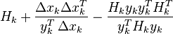 |
| BFGS | 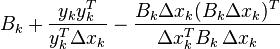 |  |
| Broyden | 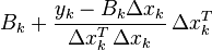 |  |
| Broyden family | ![(1-\varphi_k) B_{k+1}^{BFGS}+ \varphi_k B_{k+1}^{DFP}, \qquad \varphi\in[0,1]](http://upload.wikimedia.org/math/f/a/0/fa0b40f635e471dac81b5ee2f76acda1.png) | |
| SR1 |  | 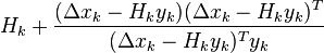 |
Other methods are Pearson's method, McCormick's Method, the Powell symmetric Broyden (PSB) method and Greenstadt's method.
Implementations
Owing to their success, there are implementations of quasi-Newton methods in almost all programming languages. The NAG Library contains several routines for minimizing or maximizing a function which use quasi-Newton algorithms.
In MATLAB's Optimization Toolbox, the fminunc function uses (among other methods) the BFGS Quasi-Newton method. Many of the constrained methods of the Optimization toolbox use BFGS and the variant L-BFGS. Many user-contributed quasi-Newton routines are available on MATLAB's file exchange.


 4042
4042

 被折叠的 条评论
为什么被折叠?
被折叠的 条评论
为什么被折叠?
 到【灌水乐园】发言


