


In applied mathematics, test functions, known as artificial landscapes, are useful to evaluate characteristics of optimization algorithms, such as:
- Velocity of convergence.
- Precision.
- Robustness.
- General performance.
Here some test functions are presented with the aim of giving an idea about the different situations that optimization algorithms have to face when coping with these kinds of problems. In the first part, some objective functions for single-objective optimization cases are presented. In the second part, test functions with their respective Pareto fronts for multi-objective optimization problems (MOP) are given.
The artificial landscapes presented herein for single-objective optimization problems are taken from Bäck,[1] Haupt et. al.[2] and from Rody Oldenhuis software.[3] Given the amount of problems (55 in total), just a few are presented here. The complete list of test functions is found on the Mathworks website.[4]
The test functions used to evaluate the algorithms for MOP were taken from Deb,[5] Binh et. al.[6] and Binh.[7] You can download the software developed by Deb,[8]which implements the NSGA-II procedure with GAs, or the program posted on Internet,[9] which implements the NSGA-II procedure with ES.
Just a general form of the equation, a plot of the objective function, boundaries of the object variables and the coordinates of global minima are given herein.
Contents
[hide]
Test functions for single-objective optimization problems[edit]
| Name | Plot | Formula | Minimum | Search domain |
|---|---|---|---|---|
| Ackley's function: | 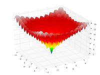 | 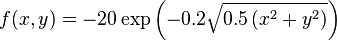
|  |  |
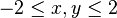
| Sphere function | 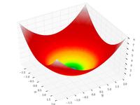 | 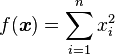 |  |  , ,  |
| Rosenbrock function | 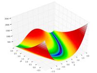 | ![f(\boldsymbol{x}) = \sum_{i=1}^{n-1} \left[ 100 \left(x_{i+1} - x_{i}^{2}\right)^{2} + \left(x_{i} - 1\right)^{2}\right]](http://upload.wikimedia.org/math/8/c/e/8ce1d6b5e80401a6df5e97bb984bb9b7.png) |  | , |
| Beale's function |  | 
|  |  |
| Goldstein–Price function: | 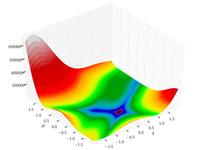 | 
|  |  |
| Booth's function: | 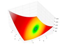 |  |  |  |
| Bukin function N.6: | 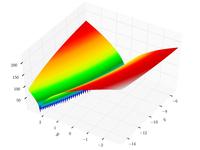 |  |  |  , ,  |
| Matyas function: | 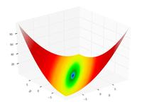 |  | | |
| Lévi function N.13: |  | 
|  | |
| Three-hump camel function: |  |  | | |
| Easom function: |  |  |  |  |
| Cross-in-tray function: | 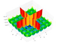 |  | 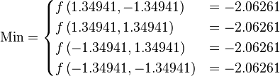 | |
| Eggholder function: | 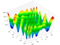 |  |  | 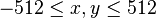 |
| Hölder table function: | 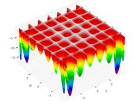 | 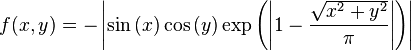 | 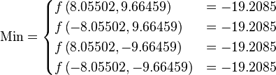 | |
| McCormick function: |  |  |  | 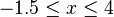 , ,  |
| Schaffer function N. 2: |  | 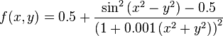 | | |
| Schaffer function N. 4: |  | 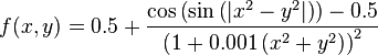 |  | |
| Styblinski–Tang function: | 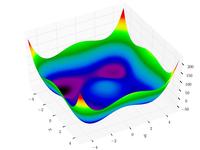 | 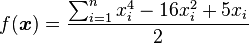 |  | 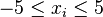 , . , . |
| Simionescu function:[10] |  |  , ,
|  |  |


Test functions for multi-objective optimization problems[edit]
| Name | Plot | Functions | Constraints | Search domain |
|---|---|---|---|---|
| Binh and Korn function: | 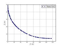 |  | 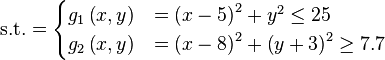 |  , ,  |
| Chakong and Haimes function: |  |  | 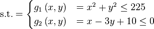 |  |
| Fonseca and Fleming function: |  |  |  , , | |
| Test function 4:[7] | ![Test function 4.[7]](http://upload.wikimedia.org/wikipedia/commons/thumb/3/3c/Test_function_4_-_Binh.pdf/page1-200px-Test_function_4_-_Binh.pdf.jpg) | 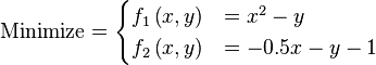 | 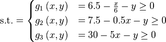 |  |
| Kursawe function: | 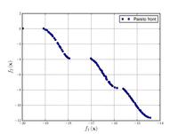 | ![\text{Minimize} =\begin{cases} f_{1}\left(\boldsymbol{x}\right) & = \sum_{i=1}^{2} \left[-10 \exp \left(-0.2 \sqrt{x_{i}^{2} + x_{i+1}^{2}} \right) \right] \\ & \\ f_{2}\left(\boldsymbol{x}\right) & = \sum_{i=1}^{3} \left[\left|x_{i}\right|^{0.8} + 5 \sin \left(x_{i}^{3} \right) \right] \\\end{cases}](http://upload.wikimedia.org/math/5/3/d/53df694c5b4d7733f3db9047108739a7.png) | ,  . . | |
| Schaffer function N. 1: |  | 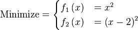 |  . Values of . Values of  form form  to to  have been used successfully. Higher values of increase the difficulty of the problem. have been used successfully. Higher values of increase the difficulty of the problem. | |
| Schaffer function N. 2: |  | 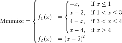 |  . . | |
| Poloni's two objective function: | 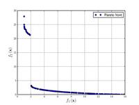 | ![\text{Minimize} =\begin{cases} f_{1}\left(x,y\right) & = \left[1 + \left(A_{1} - B_{1}\left(x,y\right) \right)^{2} + \left(A_{2} - B_{2}\left(x,y\right) \right)^{2} \right] \\ f_{2}\left(x,y\right) & = \left(x + 3\right)^{2} + \left(y + 1 \right)^{2} \\\end{cases}](http://upload.wikimedia.org/math/f/f/d/ffd85ecde4700b0d4a5834389fa6f492.png)
|  | |
| Zitzler–Deb–Thiele's function N. 1: |  |  |  , ,  . . | |
| Zitzler–Deb–Thiele's function N. 2: | 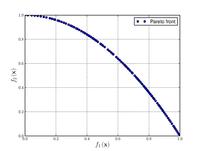 |  | , . | |
| Zitzler–Deb–Thiele's function N. 3: | 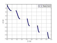 | 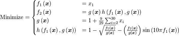 | , . | |
| Zitzler–Deb–Thiele's function N. 4: | 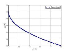 |  |  , , , ,  | |
| Zitzler–Deb–Thiele's function N. 6: |  | ![\text{Minimize} =\begin{cases} f_{1}\left(\boldsymbol{x}\right) & = 1 - \exp \left(-4x_{1}\right)\sin^{6}\left(6 \pi x_{1} \right) \\ f_{2}\left(\boldsymbol{x}\right) & = g\left(\boldsymbol{x}\right) h \left(f_{1}\left(\boldsymbol{x}\right),g\left(\boldsymbol{x}\right)\right) \\ g\left(\boldsymbol{x}\right) & = 1 + 9 \left[\frac{\sum_{i=2}^{10} x_{i}}{9}\right]^{0.25} \\ h \left(f_{1}\left(\boldsymbol{x}\right),g\left(\boldsymbol{x}\right)\right) & = 1 - \left(\frac{f_{1}\left(\boldsymbol{x}\right)}{g\left(\boldsymbol{x} \right)}\right)^{2} \\\end{cases}](http://upload.wikimedia.org/math/8/5/a/85a057897bdc21201097a9ad2396ace8.png) | ,  . . | |
| Viennet function: | 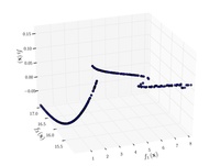 | 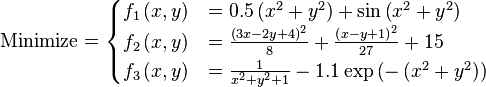 | 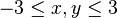 . . | |
| Osyczka and Kundu function: | 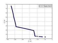 |  | 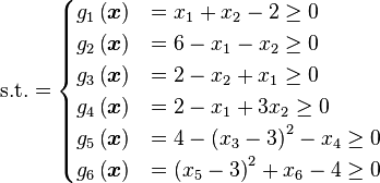 |  , , 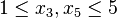 , ,  . . |
| CTP1 function (2 variables):[5] | ![CTP1 function (2 variables).[5]](http://upload.wikimedia.org/wikipedia/commons/thumb/d/d4/CTP1_function_%282_variables%29.pdf/page1-200px-CTP1_function_%282_variables%29.pdf.jpg) |  |  | 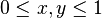 . . |
| Constr-Ex problem:[5] | ![Constr-Ex problem.[5]](http://upload.wikimedia.org/wikipedia/commons/thumb/6/6f/Constr-Ex_problem.pdf/page1-200px-Constr-Ex_problem.pdf.jpg) |  | 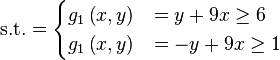 |  , ,  |

See also[edit]
- Himmelblau's function
- Rosenbrock function
- Rastrigin function
- Shekel function
- MOEA Framework, an open source Java library for multiobjective optimization
References[edit]
- Jump up^ Bäck, Thomas (1995). Evolutionary algorithms in theory and practice : evolution strategies, evolutionary programming, genetic algorithms. Oxford: Oxford University Press. p. 328. ISBN 0-19-509971-0.
- Jump up^ Haupt, Randy L. Haupt, Sue Ellen (2004). Practical genetic algorithms with DC-Rom (2nd ed. ed.). New York: J. Wiley. ISBN 0-471-45565-2.
- Jump up^ Oldenhuis, Rody. "Many test functions for global optimizers". Mathworks. Retrieved 1 November 2012.
- Jump up^ Ortiz, Gilberto A. "Evolution Strategies (ES)". Mathworks. Retrieved 1 November 2012.
- ^ Jump up to:a b c d e Deb, Kalyanmoy (2002) Multiobjective optimization using evolutionary algorithms (Repr. ed.). Chichester [u.a.]: Wiley. ISBN 0-471-87339-X.
- Jump up^ Binh T. and Korn U. (1997) MOBES: A Multiobjective Evolution Strategy for Constrained Optimization Problems. In: Proceedings of the Third International Conference on Genetic Algorithms. Czech Republic. pp. 176-182
- ^ Jump up to:a b c Binh T. (1999) A multiobjective evolutionary algorithm. The study cases. Technical report. Institute for Automation and Communication. Barleben, Germany
- Jump up^ Deb K. (2011) Software for multi-objective NSGA-II code in C. Available at URL:http://www.iitk.ac.in/kangal/codes.shtml. Revision 1.1.6
- Jump up^ Ortiz, Gilberto A. "Multi-objective optimization using ES as Evolutionary Algorithm.". Mathworks. Retrieved 1 November 2012.
- Jump up^ Simionescu, P.A. (2014). Computer Aided Graphing and Simulation Tools for AutoCAD users (1st ed.). Boca Raton, FL: CRC Press. ISBN 9-781-48225290-3.


 3474
3474

 被折叠的 条评论
为什么被折叠?
被折叠的 条评论
为什么被折叠?
 到【灌水乐园】发言


