Multiple Input and Output Models in keras

Multiple Input and Output Models

The functional API can also be used to develop more complex models with multiple inputs, possibly with different modalities. It can also be used to develop models that produce multiple outputs.

We will look at examples of each in this section.

Multiple Input Model

We will develop an image classification model that takes two versions of the image as input, each of a different size. Specifically a black and white 64×64 version and a color 32×32 version. Separate feature extraction CNN models operate on each, then the results from both models are concatenated for interpretation and ultimate prediction.

Note that in the creation of the Model() instance, that we define the two input layers as an array. Specifically:

 

1	model = Model(inputs=[visible1, visible2], outputs=output)

The complete example is listed below.

 

1 2 3 4 5 6 7 8 9 10 11 12 13 14 15 16 17 18 19 20 21 22 23 24 25 26 27 28 29 30 31 32 33 34

# Multiple Inputs from keras.utils import plot_model from keras.models import Model from keras.layers import Input from keras.layers import Dense from keras.layers import Flatten from keras.layers.convolutional import Conv2D from keras.layers.pooling import MaxPooling2D from keras.layers.merge import concatenate # first input model visible1 = Input(shape=(64,64,1)) conv11 = Conv2D(32, kernel_size=4, activation='relu')(visible1) pool11 = MaxPooling2D(pool_size=(2, 2))(conv11) conv12 = Conv2D(16, kernel_size=4, activation='relu')(pool11) pool12 = MaxPooling2D(pool_size=(2, 2))(conv12) flat1 = Flatten()(pool12) # second input model visible2 = Input(shape=(32,32,3)) conv21 = Conv2D(32, kernel_size=4, activation='relu')(visible2) pool21 = MaxPooling2D(pool_size=(2, 2))(conv21) conv22 = Conv2D(16, kernel_size=4, activation='relu')(pool21) pool22 = MaxPooling2D(pool_size=(2, 2))(conv22) flat2 = Flatten()(pool22) # merge input models merge = concatenate([flat1, flat2]) # interpretation model hidden1 = Dense(10, activation='relu')(merge) hidden2 = Dense(10, activation='relu')(hidden1) output = Dense(1, activation='sigmoid')(hidden2) model = Model(inputs=[visible1, visible2], outputs=output) # summarize layers print(model.summary()) # plot graph plot_model(model, to_file='multiple_inputs.png')

Running the example summarizes the model layers.

 

1 2 3 4 5 6 7 8 9 10 11 12 13 14 15 16 17 18 19 20 21 22 23 24 25 26 27 28 29 30 31 32 33 34 35 36 37 38 39 40

____________________________________________________________________________________________________ Layer (type)                     Output Shape          Param #     Connected to ==================================================================================================== input_1 (InputLayer)             (None, 64, 64, 1)     0 ____________________________________________________________________________________________________ input_2 (InputLayer)             (None, 32, 32, 3)     0 ____________________________________________________________________________________________________ conv2d_1 (Conv2D)                (None, 61, 61, 32)    544         input_1[0][0] ____________________________________________________________________________________________________ conv2d_3 (Conv2D)                (None, 29, 29, 32)    1568        input_2[0][0] ____________________________________________________________________________________________________ max_pooling2d_1 (MaxPooling2D)   (None, 30, 30, 32)    0           conv2d_1[0][0] ____________________________________________________________________________________________________ max_pooling2d_3 (MaxPooling2D)   (None, 14, 14, 32)    0           conv2d_3[0][0] ____________________________________________________________________________________________________ conv2d_2 (Conv2D)                (None, 27, 27, 16)    8208        max_pooling2d_1[0][0] ____________________________________________________________________________________________________ conv2d_4 (Conv2D)                (None, 11, 11, 16)    8208        max_pooling2d_3[0][0] ____________________________________________________________________________________________________ max_pooling2d_2 (MaxPooling2D)   (None, 13, 13, 16)    0           conv2d_2[0][0] ____________________________________________________________________________________________________ max_pooling2d_4 (MaxPooling2D)   (None, 5, 5, 16)      0           conv2d_4[0][0] ____________________________________________________________________________________________________ flatten_1 (Flatten)              (None, 2704)          0           max_pooling2d_2[0][0] ____________________________________________________________________________________________________ flatten_2 (Flatten)              (None, 400)           0           max_pooling2d_4[0][0] ____________________________________________________________________________________________________ concatenate_1 (Concatenate)      (None, 3104)          0           flatten_1[0][0]                                                                    flatten_2[0][0] ____________________________________________________________________________________________________ dense_1 (Dense)                  (None, 10)            31050       concatenate_1[0][0] ____________________________________________________________________________________________________ dense_2 (Dense)                  (None, 10)            110         dense_1[0][0] ____________________________________________________________________________________________________ dense_3 (Dense)                  (None, 1)             11          dense_2[0][0] ==================================================================================================== Total params: 49,699 Trainable params: 49,699 Non-trainable params: 0 ____________________________________________________________________________________________________

A plot of the model graph is also created and saved to file.

​

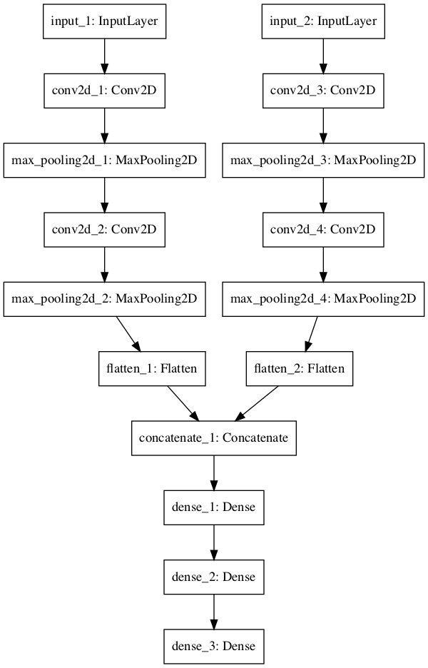
Neural Network Graph With Multiple Inputs

Multiple Output Model

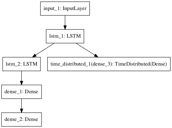
In this section, we will develop a model that makes two different types of predictions. Given an input sequence of 100 time steps of one feature, the model will both classify the sequence and output a new sequence with the same length.

An LSTM layer interprets the input sequence and returns the hidden state for each time step. The first output model creates a stacked LSTM, interprets the features, and makes a binary prediction. The second output model uses the same output layer to make a real-valued prediction for each input time step.

 

1 2 3 4 5 6 7 8 9 10 11 12 13 14 15 16 17 18 19 20 21 22 23

# Multiple Outputs from keras.utils import plot_model from keras.models import Model from keras.layers import Input from keras.layers import Dense from keras.layers.recurrent import LSTM from keras.layers.wrappers import TimeDistributed # input layer visible = Input(shape=(100,1)) # feature extraction extract = LSTM(10, return_sequences=True)(visible) # classification output class11 = LSTM(10)(extract) class12 = Dense(10, activation='relu')(class11) output1 = Dense(1, activation='sigmoid')(class12) # sequence output output2 = TimeDistributed(Dense(1, activation='linear'))(extract) # output model = Model(inputs=visible, outputs=[output1, output2]) # summarize layers print(model.summary()) # plot graph plot_model(model, to_file='multiple_outputs.png')

Running the example summarizes the model layers.

 

1 2 3 4 5 6 7 8 9 10 11 12 13 14 15 16 17 18 19

____________________________________________________________________________________________________ Layer (type)                     Output Shape          Param #     Connected to ==================================================================================================== input_1 (InputLayer)             (None, 100, 1)        0 ____________________________________________________________________________________________________ lstm_1 (LSTM)                    (None, 100, 10)       480         input_1[0][0] ____________________________________________________________________________________________________ lstm_2 (LSTM)                    (None, 10)            840         lstm_1[0][0] ____________________________________________________________________________________________________ dense_1 (Dense)                  (None, 10)            110         lstm_2[0][0] ____________________________________________________________________________________________________ dense_2 (Dense)                  (None, 1)             11          dense_1[0][0] ____________________________________________________________________________________________________ time_distributed_1 (TimeDistribu (None, 100, 1)        11          lstm_1[0][0] ==================================================================================================== Total params: 1,452 Trainable params: 1,452 Non-trainable params: 0 ____________________________________________________________________________________________________

A plot of the model graph is also created and saved to file.