RANSAC算法理解

athrunsunny

已于 2024-05-23 09:08:03 修改

阅读量1.9k

点赞数 8

分类专栏： SLAM 文章标签：算法

于 2024-05-21 21:20:04 首次发布

本文链接：https://blog.csdn.net/athrunsunny/article/details/139101287

版权

SLAM 专栏收录该内容

5 篇文章

订阅专栏

算法基本介绍

RANSAC(RAndom SAmple Consensus，随机采样一致)是一种随机参数估计算法，常常应用于二维图像的拟合、分割等等，由于是估计数学模型参数的迭代算法，因此也被用于三维平面、球的估计。

RANSAC算法由Fischler和Bolles于1981年提出，是一种从数据集合中迭代稳健估计模型参数的方法。该算法的基本思想是不断地从数据集合中随机抽取样本集，寻求支持更多局内点的模型参数，然后利用模型余集检验获得的模型参数，通过一定次数的迭代来达到最大的一致性概率，并将该采样样本集作为理解的样本集，且参数解的正确性由样本余集检验支撑。其中数据集合中包含正确数据（即内点inliers）和异常数据（外点outliers）在关键点匹配中为误匹配的点。同时RANSAC假设：在给定一组含有少部分“内点”的数据，存在一个程序可以估计出符合“内点”的模型。

RANSAC与最小二乘拟合不同，最小二乘法考虑整个数据集合中所有的数据，让数据集整体的误差最小，而RANSAC首先假设数据整体具有统一共性（即符合某个模型），为了达到这一共性，可以适当的排除一些数据，为了解决样本中外点的影响，最多可以处理50%的外点情况。

图片来源

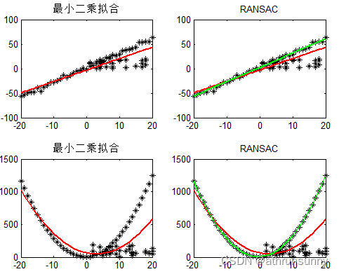
上图中给出了一阶与二阶曲线使用最小二乘法以及RANSAC拟合的效果对比。

算法思想

RANSAC算法的输入：一组观测数据，一个可以解释或者适应于观测数据的参数化模型，一些可信的参数。

RANSAC通过反复选择数据中的一组随机子集来达成目标。被选取的子集被假设为局内点，并用下述方法进行验证：

1.有一个模型适应于假设的内点，即所有的未知参数都能从假设的内点计算得出。

2.用1中得到的模型去测试所有的其它数据，如果某个点适用于估计的模型，认为它也是内点。

3.如果有足够多的点被归类为假设的内点，那么估计的模型就足够合理。

4.然后，用所有假设的内点去重新估计模型，因为它仅仅被初始的假设内点估计过。

5.最后，通过估计内点与模型的错误率来评估模型。

这个过程被重复执行固定的次数，每次产生的模型要么因为内点太少而被舍弃，要么因为比现有的模型更好而被选用。

举一个实际例子：

1）给定一个数据集 $S$ ，从中选择建立模型所需的最小样本数（例如直线最少由两个点确定，所以最小样本数是2，而平面可以根据不共线三点确定，所以最小样本数为3），记选择数据集为 $S_{1}$ ；

2）使用选择的数据集 $S$ 计算得到一个数学模型 $M$ ；

3）用计算的模型 $M$ 去测试数据集中剩余的点，如果测试的数据点在误差允许的范围内，则将该数据点判为内点（inlier），否则判为外点（outlier），记所有内点组成的数据集为 $S^{*}$ ，表示为 $S_{1}$ 的一致性集合；

4）比较当前模型和之前推出的最好的模型的“内点”的数量，记录最大“内点”数量时模型参数和“内点”数量；

5）重复1-4步，直到迭代结束或者当前模型已经足够好了（“内点数目大于设定的阈值”）。

迭代的次数可通过以下方式估计出来：

假设内点在数据集中的占比为 $p$ ，可表示为 $p = \frac{n_{inliers}}{n_{inliers}+n_{outliers}}$ ，那么我们每次计算模型使用 $k$ 个点的情况下，选取的点至少有一个外点的情况(采样失败的概率）就是 $1-p^{k}$ , 那么 $m$ 次迭代计算模型都至少采样到一个外点的概率为 $(1-p^{k})^{m}$ ，那么 $m$ 次采样至少有一次成功的概率记为 $z = 1-(1-p^{k})^{m}$ ，通过 $z$ 变换并在等式两边同时取对数可以得到 $m = \frac{log(1-z)}{log(1-p^{k})}$ 。在基本子集的迭代次数内，至少有一次采样使得采样子集内的 $k$ 个点均为内点，从而保证在迭代次数中，至少存在一次采样能够取得目标函数的最大值，因此终止循环条件应满足 $m \geq \frac{log(1-z)}{log(1-p^{k})}$ 。

内点的占比 $p$ 是一个先验值，如果一开始不知道这个先验值 $p$ ，可以采用自适应迭代的方法，用当前的内点的比值来当成 $p$ 来估算迭代的次数。然后通过不断迭代，内点的比值也逐渐增大，再用新的更大的内点比值去代替 $p$ 的值。

Pseudocode

伪代码参考自wiki

Given:
    data – A set of observations.
    model – A model to explain the observed data points.
    n – The minimum number of data points required to estimate the model parameters.
    k – The maximum number of iterations allowed in the algorithm.
    t – A threshold value to determine data points that are fit well by the model (inlier).
    d – The number of close data points (inliers) required to assert that the model fits well to the data.

Return:
    bestFit – The model parameters which may best fit the data (or null if no good model is found).


iterations = 0
bestFit = null
bestErr = something really large // This parameter is used to sharpen the model parameters to the best data fitting as iterations go on.

while iterations < k do
    maybeInliers := n randomly selected values from data
    maybeModel := model parameters fitted to maybeInliers
    confirmedInliers := empty set
    for every point in data do
        if point fits maybeModel with an error smaller than t then
             add point to confirmedInliers
        end if
    end for
    if the number of elements in confirmedInliers is > d then
        // This implies that we may have found a good model.
        // Now test how good it is.
        betterModel := model parameters fitted to all the points in confirmedInliers
        thisErr := a measure of how well betterModel fits these points
        if thisErr < bestErr then
            bestFit := betterModel
            bestErr := thisErr
        end if
    end if
    increment iterations
end while

return bestFit

python demo

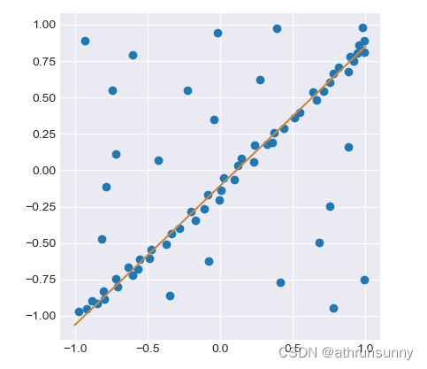
定义模型为2D线性回归模型

from copy import copy
import numpy as np
from numpy.random import default_rng

rng = default_rng()


class RANSAC:
    def __init__(self, n=10, k=100, t=0.05, d=10, model=None, loss=None, metric=None):
        self.n = n  # `n`: Minimum number of data points to estimate parameters
        self.k = k  # `k`: Maximum iterations allowed
        self.t = t  # `t`: Threshold value to determine if points are fit well
        self.d = d  # `d`: Number of close data points required to assert model fits well
        self.model = model  # `model`: class implementing `fit` and `predict`
        self.loss = loss  # `loss`: function of `y_true` and `y_pred` that returns a vector
        self.metric = metric  # `metric`: function of `y_true` and `y_pred` and returns a float
        self.best_fit = None
        self.best_error = np.inf

    def fit(self, X, y):
        for _ in range(self.k):
            ids = rng.permutation(X.shape[0])

            maybe_inliers = ids[: self.n]
            maybe_model = copy(self.model).fit(X[maybe_inliers], y[maybe_inliers])

            thresholded = (
                    self.loss(y[ids][self.n:], maybe_model.predict(X[ids][self.n:]))
                    < self.t
            )

            inlier_ids = ids[self.n:][np.flatnonzero(thresholded).flatten()]

            if inlier_ids.size > self.d:
                inlier_points = np.hstack([maybe_inliers, inlier_ids])
                better_model = copy(self.model).fit(X[inlier_points], y[inlier_points])

                this_error = self.metric(
                    y[inlier_points], better_model.predict(X[inlier_points])
                )

                if this_error < self.best_error:
                    self.best_error = this_error
                    self.best_fit = better_model

        return self

    def predict(self, X):
        return self.best_fit.predict(X)


def square_error_loss(y_true, y_pred):
    return (y_true - y_pred) ** 2


def mean_square_error(y_true, y_pred):
    return np.sum(square_error_loss(y_true, y_pred)) / y_true.shape[0]


class LinearRegressor:
    def __init__(self):
        self.params = None

    def fit(self, X: np.ndarray, y: np.ndarray):
        r, _ = X.shape
        X = np.hstack([np.ones((r, 1)), X])
        self.params = np.linalg.inv(X.T @ X) @ X.T @ y
        return self

    def predict(self, X: np.ndarray):
        r, _ = X.shape
        X = np.hstack([np.ones((r, 1)), X])
        return X @ self.params


if __name__ == "__main__":
    regressor = RANSAC(model=LinearRegressor(), loss=square_error_loss, metric=mean_square_error)

    X = np.array(
        [-0.848, -0.800, -0.704, -0.632, -0.488, -0.472, -0.368, -0.336, -0.280, -0.200, -0.00800, -0.0840, 0.0240,
         0.100, 0.124, 0.148, 0.232, 0.236, 0.324, 0.356, 0.368, 0.440, 0.512, 0.548, 0.660, 0.640, 0.712, 0.752, 0.776,
         0.880, 0.920, 0.944, -0.108, -0.168, -0.720, -0.784, -0.224, -0.604, -0.740, -0.0440, 0.388, -0.0200, 0.752,
         0.416, -0.0800, -0.348, 0.988, 0.776, 0.680, 0.880, -0.816, -0.424, -0.932, 0.272, -0.556, -0.568, -0.600,
         -0.716, -0.796, -0.880, -0.972, -0.916, 0.816, 0.892, 0.956, 0.980, 0.988, 0.992, 0.00400]).reshape(-1, 1)
    y = np.array(
        [-0.917, -0.833, -0.801, -0.665, -0.605, -0.545, -0.509, -0.433, -0.397, -0.281, -0.205, -0.169, -0.0531,
         -0.0651, 0.0349, 0.0829, 0.0589, 0.175, 0.179, 0.191, 0.259, 0.287, 0.359, 0.395, 0.483, 0.539, 0.543, 0.603,
         0.667, 0.679, 0.751, 0.803, -0.265, -0.341, 0.111, -0.113, 0.547, 0.791, 0.551, 0.347, 0.975, 0.943, -0.249,
         -0.769, -0.625, -0.861, -0.749, -0.945, -0.493, 0.163, -0.469, 0.0669, 0.891, 0.623, -0.609, -0.677, -0.721,
         -0.745, -0.885, -0.897, -0.969, -0.949, 0.707, 0.783, 0.859, 0.979, 0.811, 0.891, -0.137]).reshape(-1, 1)

    regressor.fit(X, y)

    import matplotlib.pyplot as plt

    plt.style.use("seaborn-darkgrid")
    fig, ax = plt.subplots(1, 1)
    ax.set_aspect(1)

    plt.scatter(X, y)

    line = np.linspace(-1, 1, num=100).reshape(-1, 1)
    plt.plot(line, regressor.predict(line), c="peru")
    plt.show()

运行可得到：