【深度学习】-Imdb数据集情感分析之模型对比（3）- CNN

你的城有我的影

已于 2022-07-15 15:23:27 修改

阅读量1.5k

点赞数 2

文章标签：深度学习 cnn 神经网络

于 2022-07-15 10:21:55 首次发布

本文链接：https://blog.csdn.net/auroro1/article/details/125796386

版权

【深度学习】-Imdb数据集情感分析之模型对比（3）- CNN

前言

【深度学习】-Imdb数据集情感分析之模型对比（2）- LSTM
【深度学习】-Imdb数据集情感分析之模型对比（1）- RNN

对之前内容感兴趣的朋友可以参考上面这两篇文章，接下来我要给大家介绍本篇博客的内容。之前引入的LSTM以及RNN两种模型都是一类有“记忆的”模型，即文本关系型特征模型，为了添加对比，我们引入了另一种文本结构化深度学习模型–CNN模型。

一，CNN是什么？

算法简介

积神经网络（CNN）是一种具有卷积计算的前向神经网络，它能根据其特殊的分类层次结构翻译输入的信息。CNN主要用于图像识别（CV）和计算机视觉方向。然而，2014年，Yoon Kim对CNN输入级别进行了一些更改，并提出了文本CNN文本分类模型。而这一次实验中，TextCNN的网络结构没有变化，甚至更简单。这一类应用于文本分类任务的CNN卷积神经网络模型，使用多个不同大小的核来提取句子中的关键信息，以便能够更好地捕捉局部相关性。

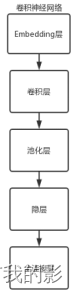
在2017年，孙松涛等使用CNN模型来对微博语料进行情感分类。我们学习了其模型架构，即在文本中，每个词都可以用一个向量表示，一句话就可以用一个矩阵来表示，那么处理文本就与处理图像是类似的了。这样我们就可以使用CNN模型运用与自然语言处理上面。该模型主要由卷积、池化和连接三层结构组成。卷积层部分负责提取文本数据局部特征；池化层部分可以用于降维；全连接层部分用于产生所需的结果。模型卷积层结构大致如图所示：
CNN卷积层结构

二、训练CNN模型

1.数据预处理

与前文类似，详细请移步【深度学习】-Imdb数据集情感分析之模型对比（1）- RNN
数据预处理部分

2.构建及训练CNN模型

模型结构

在这里插入图片描述

设定模型参数

max_features = 4000  # 最大特征数（词汇表大小）
maxlen = 400         # 序列最大长度
batch_size = 32      # 每批数据量大小
embedding_dims = 32  # 词嵌入维度
nb_filter = 32      # 1维卷积核个数
filter_length = 5    # 卷积核长度
hidden_dims = 256    # 隐藏层维度
nb_epoch =10       # 迭代次数

构建网络模型

model = Sequential()
# 先从一个高效的嵌入层开始，它将词汇的索引值映射为 embedding_dims 维度的词向量
model.add(Embedding(max_features,
                    embedding_dims,
                    input_length=maxlen,
# 添加一个 1D 卷积层，它将学习 nb_filter 个 filter_length 大小的词组卷积核
model.add(Convolution1D(nb_filter=nb_filter,
                        filter_length=filter_length,
                        border_mode='valid',
                        activation='relu',
                        subsample_length=1))
model.add(Dropout(0.2))
# 使用最大池化
model.add(GlobalMaxPooling1D()) 
# 添加一个原始隐藏层
model.add(Dense(hidden_dims))
model.add(Activation('relu'))
# 投影到一个单神经元的输出层，并且使用 sigmoid 压缩它
model.add(Dense(1))
model.add(Activation('sigmoid'))
model.summary()  # 模型概述

训练模型

定义损失函数，优化器以及评估矩阵，并开始训练模型。

# 定义损失函数，优化器，评估矩阵
model.compile(loss='binary_crossentropy',
              optimizer='adam',
              metrics=['accuracy'])
 
# 训练，迭代 nb_epoch 次

train_history =model.fit(x_train, y_train,
          batch_size=batch_size,
          nb_epoch=nb_epoch,
          validation_data=(x_test, y_test))

开始训练

Epoch 1/10
25000/25000 [==============================] - 26s 1ms/step - loss: 0.4127 - accuracy: 0.7950 - val_loss: 0.2981 - val_accuracy: 0.8759
Epoch 2/10
25000/25000 [==============================] - 25s 991us/step - loss: 0.2207 - accuracy: 0.9117 - val_loss: 0.2846 - val_accuracy: 0.8803
Epoch 3/10
25000/25000 [==============================] - 25s 983us/step - loss: 0.1388 - accuracy: 0.9496 - val_loss: 0.2919 - val_accuracy: 0.8807
Epoch 4/10
25000/25000 [==============================] - 25s 989us/step - loss: 0.0864 - accuracy: 0.9682 - val_loss: 0.3275 - val_accuracy: 0.8792
Epoch 5/10
25000/25000 [==============================] - 25s 985us/step - loss: 0.0543 - accuracy: 0.9809 - val_loss: 0.3874 - val_accuracy: 0.8764
Epoch 6/10
25000/25000 [==============================] - 25s 986us/step - loss: 0.0443 - accuracy: 0.9838 - val_loss: 0.5893 - val_accuracy: 0.8457
Epoch 7/10
25000/25000 [==============================] - 25s 987us/step - loss: 0.0368 - accuracy: 0.9863 - val_loss: 0.4689 - val_accuracy: 0.8719
Epoch 8/10
25000/25000 [==============================] - 25s 987us/step - loss: 0.0335 - accuracy: 0.9880 - val_loss: 0.4722 - val_accuracy: 0.8755
Epoch 9/10
25000/25000 [==============================] - 25s 1ms/step - loss: 0.0348 - accuracy: 0.9873 - val_loss: 0.4722 - val_accuracy: 0.8752
Epoch 10/10
25000/25000 [==============================] - 25s 993us/step - loss: 0.0276 - accuracy: 0.9899 - val_loss: 0.4738 - val_accuracy: 0.8752

三、可视化结果

import matplotlib.pyplot as plt
def show_train_history(train_history,train,validation):
    plt.plot(train_history.history[train])
    plt.plot(train_history.history[validation])
    plt.title('Train History')
    plt.ylabel(train)
    plt.xlabel('Epoch')
    plt.legend(['train', 'validation'], loc='upper left')
    plt.show()
 
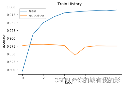
show_train_history(train_history,'accuracy','val_accuracy')
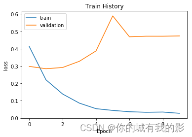
show_train_history(train_history,'loss','val_loss')
print('Test score:', score)
print('Test accuracy:', acc)

在这里插入图片描述

✿四、模型预测

前几节都忘记加上这一板块了，加在本篇里面。
（主要还是博主太懒了，下次一定。）

在这里我们使用训练好的模型对测试集进行预测

#####预测结果
predict=model.predict_classes(x_test)
 
predict[:10]
predict.shape
predict_classes=predict.reshape(25000)

print(predict_classes)
#
SentimentDict={1:'正面的',0:'负面的'}
def display_test_Sentiment(i):
    print(test_text[i])
    print('label真实值:',SentimentDict[y_test[i]],
          '预测结果:',SentimentDict[predict_classes[i]])

当然我们可以把他写成一个方法体，方便下次预测其他数据集时进行调用。

display_test_Sentiment(28)

# 
def predict_review(input_text):
    input_seq = token.texts_to_sequences([input_text])
    pad_input_seq  = sequence.pad_sequences(input_seq , maxlen=400)
    predict_result=model.predict_classes(pad_input_seq)
    print(SentimentDict[predict_result[0][0]])

我们实现准备好了一段正向的英文影评数据用于测试

#正面

predict_review('''
The original Beauty and the Beast was my favorite cartoon as a kid but it did have major plot holes. Why had no one else ever seen the castle or knew where it was? Didn't anyone miss the people who were cursed? All of that gets an explanation when the enchantress places her curse in the beginning. Why did Belle and her Father move to a small town? Her mother died and the father thought it as best to leave. I love the new songs and added lyrics to the originals. I like the way the cgi beast looks (just the face is CGi). I think Emma Watson is a perfect Belle who is outspoken, fearless, and different. The set design is perfect for the era in France.
I know a lot of people disagree but I found this remake with all its changes to be more enchanting, beautiful, and complete than the original 1991 movie. To each his own but I think everyone should see it for themselves. 
''')

无论是使用测试集的例子还是我们引入的新影评数据，都得到了我们想要的预测结果
label真实值: 正面的预测结果: 正面的正面的

五、评估模型并保存

模型评估

用测试集对模型的匹配精度进行评估

score, acc = model.evaluate(x_test, y_test,
                            batch_size=128)

保存模型

model_json = model.to_json()
with open("D:/final_all/1/1.json", "w") as json_file:
    json_file.write(model_json)

model.save_weights("D:/final_all/1/2.h5")
print("Saved model to disk")