吴恩达深度学习笔记 cousrse4 week1作业

Convolutional Neural Networks: Step by Step¶

Welcome to Course 4's first assignment! In this assignment, you will implement convolutional (CONV) and pooling (POOL) layers in numpy, including both forward propagation and (optionally) backward propagation.

Notation:

• Superscript [l][l] denotes an object of the lthlth layer.
  • Example: a[4]a[4] is the 4th4th layer activation. W[5]W[5] and b[5]b[5] are the 5th5th layer parameters.

• Superscript (i)(i) denotes an object from the ithith example.
  • Example: x(i)x(i) is the ithith training example input.

• Lowerscript ii denotes the ithith entry of a vector.
  • Example: a[l]iai[l] denotes the ithith entry of the activations in layer ll, assuming this is a fully connected (FC) layer.

• nHnH, nWnW and nCnC denote respectively the height, width and number of channels of a given layer. If you want to reference a specific layer ll, you can also write n[l]HnH[l], n[l]WnW[l], n[l]CnC[l].
• nHprevnHprev, nWprevnWprev and nCprevnCprev denote respectively the height, width and number of channels of the previous layer. If referencing a specific layer ll, this could also be denoted n[l−1]HnH[l−1], n[l−1]WnW[l−1], n[l−1]CnC[l−1].

We assume that you are already familiar with numpy and/or have completed the previous courses of the specialization. Let's get started!

 

1 - Packages

Let's first import all the packages that you will need during this assignment.

• numpy is the fundamental package for scientific computing with Python.
• matplotlib is a library to plot graphs in Python.
• np.random.seed(1) is used to keep all the random function calls consistent. It will help us grade your work.

In [43]:

 

 

 

 

 

import numpy as np

import h5py

import matplotlib.pyplot as plt

​

%matplotlib inline

plt.rcParams['figure.figsize'] = (5.0, 4.0) # set default size of plots

plt.rcParams['image.interpolation'] = 'nearest'

plt.rcParams['image.cmap'] = 'gray'

​

%load_ext autoreload

%autoreload 2

​

np.random.seed(1)

 

 

 

The autoreload extension is already loaded. To reload it, use:
  %reload_ext autoreload

 

2 - Outline of the Assignment

You will be implementing the building blocks of a convolutional neural network! Each function you will implement will have detailed instructions that will walk you through the steps needed:

• Convolution functions, including:
  • Zero Padding
  • Convolve window
  • Convolution forward
  • Convolution backward (optional)
• Pooling functions, including:
  • Pooling forward
  • Create mask
  • Distribute value
  • Pooling backward (optional)

This notebook will ask you to implement these functions from scratch in numpy. In the next notebook, you will use the TensorFlow equivalents of these functions to build the following model:

Note that for every forward function, there is its corresponding backward equivalent. Hence, at every step of your forward module you will store some parameters in a cache. These parameters are used to compute gradients during backpropagation.

 

3 - Convolutional Neural Networks

Although programming frameworks make convolutions easy to use, they remain one of the hardest concepts to understand in Deep Learning. A convolution layer transforms an input volume into an output volume of different size, as shown below.

In this part, you will build every step of the convolution layer. You will first implement two helper functions: one for zero padding and the other for computing the convolution function itself.

 

3.1 - Zero-Padding

Zero-padding adds zeros around the border of an image:

Figure 1  : Zero-Padding
Image (3 channels, RGB) with a padding of 2.

The main benefits of padding are the following:

• It allows you to use a CONV layer without necessarily shrinking the height and width of the volumes. This is important for building deeper networks, since otherwise the height/width would shrink as you go to deeper layers. An important special case is the "same" convolution, in which the height/width is exactly preserved after one layer.

• It helps us keep more of the information at the border of an image. Without padding, very few values at the next layer would be affected by pixels as the edges of an image.

Exercise: Implement the following function, which pads all the images of a batch of examples X with zeros. Use np.pad. Note if you want to pad the array "a" of shape (5,5,5,5,5)(5,5,5,5,5) with pad = 1 for the 2nd dimension, pad = 3 for the 4th dimension and pad = 0 for the rest, you would do:

a = np.pad(a, ((0,0), (1,1), (0,0), (3,3), (0,0)), 'constant', constant_values = (..,..)) 

In [44]:

 

 

 

 

 

# GRADED FUNCTION: zero_pad

​

def zero_pad(X, pad):

    """

    Pad with zeros all images of the dataset X. The padding is applied to the height and width of an image, 

    as illustrated in Figure 1.

    Argument:

    X -- python numpy array of shape (m, n_H, n_W, n_C) representing a batch of m images

    pad -- integer, amount of padding around each image on vertical and horizontal dimensions

    Returns:

    X_pad -- padded image of shape (m, n_H + 2*pad, n_W + 2*pad, n_C)

    """

    ### START CODE HERE ### (≈ 1 line)

    X_pad = np.pad(X,

                   ((0,0),

                    (pad,pad),

                    (pad,pad),

                    (0,0)),

                   'constant',

                   constant_values=0

                  )

    ### END CODE HERE ###

    return X_pad

 

 

In [45]:

 

 

 

 

 

np.random.seed(1)

x = np.random.randn(4, 3, 3, 2)

x_pad = zero_pad(x, 2)

print ("x.shape =", x.shape)

print ("x_pad.shape =", x_pad.shape)

print ("x[1,1] =", x[1,1])

print ("x_pad[1,1] =", x_pad[1,1])

​

fig, axarr = plt.subplots(1, 2)

axarr[0].set_title('x')

axarr[0].imshow(x[0,:,:,0])

axarr[1].set_title('x_pad')

axarr[1].imshow(x_pad[0,:,:,0])

 

 

 

x.shape = (4, 3, 3, 2)
x_pad.shape = (4, 7, 7, 2)
x[1,1] = [[ 0.90085595 -0.68372786]
 [-0.12289023 -0.93576943]
 [-0.26788808  0.53035547]]
x_pad[1,1] = [[ 0.  0.]
 [ 0.  0.]
 [ 0.  0.]
 [ 0.  0.]
 [ 0.  0.]
 [ 0.  0.]
 [ 0.  0.]]

Out[45]:

<matplotlib.image.AxesImage at 0x7f14a032cdd8>

 

 

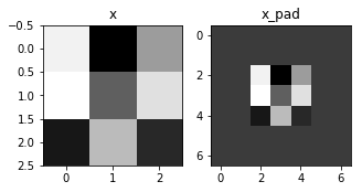
Expected Output:

x.shape:	(4, 3, 3, 2)
x_pad.shape:	(4, 7, 7, 2)
x[1,1]:	[[ 0.90085595 -0.68372786] [-0.12289023 -0.93576943] [-0.26788808 0.53035547]]
x_pad[1,1]:	[[ 0. 0.] [ 0. 0.] [ 0. 0.] [ 0. 0.] [ 0. 0.] [ 0. 0.] [ 0. 0.]]

 

3.2 - Single step of convolution

In this part, implement a single step of convolution, in which you apply the filter to a single position of the input. This will be used to build a convolutional unit, which:

• Takes an input volume
• Applies a filter at every position of the input
• Outputs another volume (usually of different size)

Figure 2  : Convolution operation
with a filter of 2x2 and a stride of 1 (stride = amount you move the window each time you slide)

In a computer vision application, each value in the matrix on the left corresponds to a single pixel value, and we convolve a 3x3 filter with the image by multiplying its values element-wise with the original matrix, then summing them up and adding a bias. In this first step of the exercise, you will implement a single step of convolution, corresponding to applying a filter to just one of the positions to get a single real-valued output.

Later in this notebook, you'll apply this function to multiple positions of the input to implement the full convolutional operation.

Exercise: Implement conv_single_step(). Hint.

In [46]:

 

 

 

 

 

# GRADED FUNCTION: conv_single_step

​

def conv_single_step(a_slice_prev, W, b):

    """

    Apply one filter defined by parameters W on a single slice (a_slice_prev) of the output activation 

    of the previous layer.

    Arguments:

    a_slice_prev -- slice of input data of shape (f, f, n_C_prev)

    W -- Weight parameters contained in a window - matrix of shape (f, f, n_C_prev)

    b -- Bias parameters contained in a window - matrix of shape (1, 1, 1)

    Returns:

    Z -- a scalar value, result of convolving the sliding window (W, b) on a slice x of the input data

    """

​

    ### START CODE HERE ### (≈ 2 lines of code)

    # Element-wise product between a_slice and W. Do not add the bias yet.

    s =np.multiply(a_slice_prev,W)

    # Sum over all entries of the volume s.

    Z =np.sum(s)

    # Add bias b to Z. Cast b to a float() so that Z results in a scalar value.

    Z =Z+b

    ### END CODE HERE ###

​

    return Z

 

 

In [47]:

 

 

 

 

 

np.random.seed(1)

a_slice_prev = np.random.randn(4, 4, 3)

W = np.random.randn(4, 4, 3)

b = np.random.randn(1, 1, 1)

​

Z = conv_single_step(a_slice_prev, W, b)

print("Z =", Z)

 

 

 

Z = [[[-6.99908945]]]

 

Expected Output:

Z	-6.99908945068

 

3.3 - Convolutional Neural Networks - Forward pass

In the forward pass, you will take many filters and convolve them on the input. Each 'convolution' gives you a 2D matrix output. You will then stack these outputs to get a 3D volume:

Exercise: Implement the function below to convolve the filters W on an input activation A_prev. This function takes as input A_prev, the activations output by the previous layer (for a batch of m inputs), F filters/weights denoted by W, and a bias vector denoted by b, where each filter has its own (single) bias. Finally you also have access to the hyperparameters dictionary which contains the stride and the padding.

Hint:

1. To select a 2x2 slice at the upper left corner of a matrix "a_prev" (shape (5,5,3)), you would do:

   a_slice_prev = a_prev[0:2,0:2,:] 

   This will be useful when you will define a_slice_prev below, using the start/end indexes you will define.
2. To define a_slice you will need to first define its corners vert_start, vert_end, horiz_start and horiz_end. This figure may be helpful for you to find how each of the corner can be defined using h, w, f and s in the code below.

Figure 3  : Definition of a slice using vertical and horizontal start/end (with a 2x2 filter) 
This figure shows only a single channel.

Reminder: The formulas relating the output shape of the convolution to the input shape is:

nH=⌊nHprev−f+2×padstride⌋+1nH=⌊nHprev−f+2×padstride⌋+1

nW=⌊nWprev−f+2×padstride⌋+1nW=⌊nWprev−f+2×padstride⌋+1

nC=number of filters used in the convolutionnC=number of filters used in the convolution

 

For this exercise, we won't worry about vectorization, and will just implement everything with for-loops.

In [48]:

 

 

 

 

 

# GRADED FUNCTION: conv_forward

​

def conv_forward(A_prev, W, b, hparameters):

    """

    Implements the forward propagation for a convolution function

    Arguments:

    A_prev -- output activations of the previous layer, numpy array of shape (m, n_H_prev, n_W_prev, n_C_prev)

    W -- Weights, numpy array of shape (f, f, n_C_prev, n_C)

    b -- Biases, numpy array of shape (1, 1, 1, n_C)

    hparameters -- python dictionary containing "stride" and "pad"

    Returns:

    Z -- conv output, numpy array of shape (m, n_H, n_W, n_C)

    cache -- cache of values needed for the conv_backward() function

    """

    ### START CODE HERE ###

    # Retrieve dimensions from A_prev's shape (≈1 line)  

    (m, n_H_prev, n_W_prev, n_C_prev) =A_prev.shape

    # Retrieve dimensions from W's shape (≈1 line)

    (f, f, n_C_prev, n_C) = W.shape

    # Retrieve information from "hparameters" (≈2 lines)

    stride =hparameters['stride']

    pad = hparameters['pad']

    # Compute the dimensions of the CONV output volume using the formula given above. Hint: use int() to floor. (≈2 lines)

    n_H = int((n_H_prev+2*pad-f)/stride)+1

    n_W =int((n_W_prev+2*pad-f)/stride)+1

    # Initialize the output volume Z with zeros. (≈1 line)

    Z = np.zeros((m,n_H,n_W,n_C))

    # Create A_prev_pad by padding A_prev

    A_prev_pad = zero_pad(A_prev, pad)

    for i in range(m):                               # loop over the batch of training examples

        a_prev_pad = A_prev_pad[i]                               # Select ith training example's padded activation

        for h in range(n_H):                           # loop over vertical axis of the output volume

            for w in range(n_W):                       # loop over horizontal axis of the output volume

                for c in range(n_C):                   # loop over channels (= #filters) of the output volume

                    # Find the corners of the current "slice" (≈4 lines)

                    vert_start = h*stride

                    vert_end = vert_start+f

                    horiz_start = w*stride

                    horiz_end = horiz_start+f

                    # Use the corners to define the (3D) slice of a_prev_pad (See Hint above the cell). (≈1 line)

                    a_slice_prev = a_prev_pad[vert_start:vert_end,horiz_start:horiz_end,:]

                    # Convolve the (3D) slice with the correct filter W and bias b, to get back one output neuron. (≈1 line)

                    Z[i, h, w, c] = conv_single_step(a_slice_prev ,W[:,:,:,c],b[:,:,0:,c])

    ### END CODE HERE ###

    # Making sure your output shape is correct

    assert(Z.shape == (m, n_H, n_W, n_C))

    # Save information in "cache" for the backprop

    cache = (A_prev, W, b, hparameters)

    return Z, cache

 

 

In [49]:

 

 

 

 

 

np.random.seed(1)

A_prev = np.random.randn(10,4,4,3)

W = np.random.randn(2,2,3,8)

b = np.random.randn(1,1,1,8)

hparameters = {"pad" : 2,

               "stride": 2}

​

Z, cache_conv = conv_forward(A_prev, W, b, hparameters)

print("Z's mean =", np.mean(Z))

print("Z[3,2,1] =", Z[3,2,1])

print("cache_conv[0][1][2][3] =", cache_conv[0][1][2][3])

 

 

 

Z's mean = 0.0489952035289
Z[3,2,1] = [-0.61490741 -6.7439236  -2.55153897  1.75698377  3.56208902  0.53036437
  5.18531798  8.75898442]
cache_conv[0][1][2][3] = [-0.20075807  0.18656139  0.41005165]

 

Expected Output:

Z's mean	0.0489952035289
Z[3,2,1]	[-0.61490741 -6.7439236 -2.55153897 1.75698377 3.56208902 0.53036437 5.18531798 8.75898442]
cache_conv[0][1][2][3]	[-0.20075807 0.18656139 0.41005165]

 

Finally, CONV layer should also contain an activation, in which case we would add the following line of code:

# Convolve the window to get back one output neuron
Z[i, h, w, c] = ... # Apply activation A[i, h, w, c] = activation(Z[i, h, w, c]) 

You don't need to do it here.

 

4 - Pooling layer

The pooling (POOL) layer reduces the height and width of the input. It helps reduce computation, as well as helps make feature detectors more invariant to its position in the input. The two types of pooling layers are:

• Max-pooling layer: slides an (f,ff,f) window over the input and stores the max value of the window in the output.

• Average-pooling layer: slides an (f,ff,f) window over the input and stores the average value of the window in the output.

These pooling layers have no parameters for backpropagation to train. However, they have hyperparameters such as the window size ff. This specifies the height and width of the fxf window you would compute a max or average over.

4.1 - Forward Pooling

Now, you are going to implement MAX-POOL and AVG-POOL, in the same function.

Exercise: Implement the forward pass of the pooling layer. Follow the hints in the comments below.

Reminder: As there's no padding, the formulas binding the output shape of the pooling to the input shape is:

nH=⌊nHprev−fstride⌋+1nH=⌊nHprev−fstride⌋+1

nW=⌊nWprev−fstride⌋+1nW=⌊nWprev−fstride⌋+1

nC=nCprevnC=nCprev

In [50]:

 

 

 

 

 

# GRADED FUNCTION: pool_forward

​

def pool_forward(A_prev, hparameters, mode = "max"):

    """

    Implements the forward pass of the pooling layer

    Arguments:

    A_prev -- Input data, numpy array of shape (m, n_H_prev, n_W_prev, n_C_prev)

    hparameters -- python dictionary containing "f" and "stride"

    mode -- the pooling mode you would like to use, defined as a string ("max" or "average")

    Returns:

    A -- output of the pool layer, a numpy array of shape (m, n_H, n_W, n_C)

    cache -- cache used in the backward pass of the pooling layer, contains the input and hparameters 

    """

    # Retrieve dimensions from the input shape

    (m, n_H_prev, n_W_prev, n_C_prev) = A_prev.shape

    # Retrieve hyperparameters from "hparameters"

    f = hparameters["f"]

    stride = hparameters["stride"]

    # Define the dimensions of the output

    n_H = int(1 + (n_H_prev - f) / stride)

    n_W = int(1 + (n_W_prev - f) / stride)

    n_C = n_C_prev

    # Initialize output matrix A

    A = np.zeros((m, n_H, n_W, n_C)) 

    ### START CODE HERE ###

    for i in range(m):                         # loop over the training examples

        for h in range(n_H):                     # loop on the vertical axis of the output volume

            for w in range(n_W):                 # loop on the horizontal axis of the output volume

                for c in range (n_C):            # loop over the channels of the output volume

                    # Find the corners of the current "slice" (≈4 lines)

                    vert_start = h*stride

                    vert_end = vert_start+f

                    horiz_start =w*stride

                    horiz_end = horiz_start+f

                    # Use the corners to define the current slice on the ith training example of A_prev, channel c. (≈1 line)

                    a_prev_slice = A_prev[i,vert_start:vert_end,horiz_start:horiz_end,c]

                    #print (a_prev_slice.shape)

                    # Compute the pooling operation on the slice. Use an if statment to differentiate the modes. Use np.max/np.mean.

                    if mode == "max":

                        A[i, h, w, c] = np.max(a_prev_slice)

                    elif mode == "average":

                        A[i, h, w, c] = np.mean(a_prev_slice)

    ### END CODE HERE ###

    # Store the input and hparameters in "cache" for pool_backward()

    cache = (A_prev, hparameters)

    # Making sure your output shape is correct

    assert(A.shape == (m, n_H, n_W, n_C))

    return A, cache

 

 

In [51]:

 

 

 

 

 

np.random.seed(1)

A_prev = np.random.randn(2, 4, 4, 3)

hparameters = {"stride" : 2, "f": 3}

​

A, cache = pool_forward(A_prev, hparameters)

print("mode = max")

print("A =", A)

print()

A, cache = pool_forward(A_prev, hparameters, mode = "average")

print("mode = average")

print("A =", A)

 

 

 

mode = max
A = [[[[ 1.74481176  0.86540763  1.13376944]]]


 [[[ 1.13162939  1.51981682  2.18557541]]]]

mode = average
A = [[[[ 0.02105773 -0.20328806 -0.40389855]]]


 [[[-0.22154621  0.51716526  0.48155844]]]]

 

Expected Output:

A =	[[[[ 1.74481176 0.86540763 1.13376944]]] [[[ 1.13162939 1.51981682 2.18557541]]]]
A =	[[[[ 0.02105773 -0.20328806 -0.40389855]]] [[[-0.22154621 0.51716526 0.48155844]]]]

 

Congratulations! You have now implemented the forward passes of all the layers of a convolutional network.

The remainer of this notebook is optional, and will not be graded.

 

5 - Backpropagation in convolutional neural networks (OPTIONAL / UNGRADED)

In modern deep learning frameworks, you only have to implement the forward pass, and the framework takes care of the backward pass, so most deep learning engineers don't need to bother with the details of the backward pass. The backward pass for convolutional networks is complicated. If you wish however, you can work through this optional portion of the notebook to get a sense of what backprop in a convolutional network looks like.

When in an earlier course you implemented a simple (fully connected) neural network, you used backpropagation to compute the derivatives with respect to the cost to update the parameters. Similarly, in convolutional neural networks you can to calculate the derivatives with respect to the cost in order to update the parameters. The backprop equations are not trivial and we did not derive them in lecture, but we briefly presented them below.

5.1 - Convolutional layer backward pass

Let's start by implementing the backward pass for a CONV layer.

5.1.1 - Computing dA:

This is the formula for computing dAdA with respect to the cost for a certain filter WcWc and a given training example:

 

dA+=∑h=0nH∑w=0nWWc×dZhw(1)(1)dA+=∑h=0nH∑w=0nWWc×dZhw

 

Where WcWc is a filter and dZhwdZhw is a scalar corresponding to the gradient of the cost with respect to the output of the conv layer Z at the hth row and wth column (corresponding to the dot product taken at the ith stride left and jth stride down). Note that at each time, we multiply the the same filter WcWc by a different dZ when updating dA. We do so mainly because when computing the forward propagation, each filter is dotted and summed by a different a_slice. Therefore when computing the backprop for dA, we are just adding the gradients of all the a_slices.

In code, inside the appropriate for-loops, this formula translates into:

da_prev_pad[vert_start:vert_end, horiz_start:horiz_end, :] += W[:,:,:,c] * dZ[i, h, w, c] 

5.1.2 - Computing dW:

This is the formula for computing dWcdWc (dWcdWc is the derivative of one filter) with respect to the loss:

 

dWc+=∑h=0nH∑w=0nWaslice×dZhw(2)(2)dWc+=∑h=0nH∑w=0nWaslice×dZhw

 

Where asliceaslice corresponds to the slice which was used to generate the acitivation ZijZij. Hence, this ends up giving us the gradient for WW with respect to that slice. Since it is the same WW, we will just add up all such gradients to get dWdW.

In code, inside the appropriate for-loops, this formula translates into:

dW[:,:,:,c] += a_slice * dZ[i, h, w, c] 

5.1.3 - Computing db:

This is the formula for computing dbdb with respect to the cost for a certain filter WcWc:

 

db=∑h∑wdZhw(3)(3)db=∑h∑wdZhw

 

As you have previously seen in basic neural networks, db is computed by summing dZdZ. In this case, you are just summing over all the gradients of the conv output (Z) with respect to the cost.

In code, inside the appropriate for-loops, this formula translates into:

db[:,:,:,c] += dZ[i, h, w, c] 

Exercise: Implement the conv_backward function below. You should sum over all the training examples, filters, heights, and widths. You should then compute the derivatives using formulas 1, 2 and 3 above.

In [52]:

 

 

 

 

 

def conv_backward(dZ, cache):

    """

    Implement the backward propagation for a convolution function

    Arguments:

    dZ -- gradient of the cost with respect to the output of the conv layer (Z), numpy array of shape (m, n_H, n_W, n_C)

    cache -- cache of values needed for the conv_backward(), output of conv_forward()

    Returns:

    dA_prev -- gradient of the cost with respect to the input of the conv layer (A_prev),

               numpy array of shape (m, n_H_prev, n_W_prev, n_C_prev)

    dW -- gradient of the cost with respect to the weights of the conv layer (W)

          numpy array of shape (f, f, n_C_prev, n_C)

    db -- gradient of the cost with respect to the biases of the conv layer (b)

          numpy array of shape (1, 1, 1, n_C)

    """

    ### START CODE HERE ###

    # Retrieve information from "cache"

    (A_prev, W, b, hparameters) = cache

    # Retrieve dimensions from A_prev's shape

    (m, n_H_prev, n_W_prev, n_C_prev) =A_prev.shape

    # Retrieve dimensions from W's shape

    (f, f, n_C_prev, n_C) = W.shape

    # Retrieve information from "hparameters"

    stride = hparameters['stride']

    pad =hparameters['pad']

    # Retrieve dimensions from dZ's shape

    (m, n_H, n_W, n_C) = dZ.shape

    # Initialize dA_prev, dW, db with the correct shapes

    dA_prev =np.zeros(A_prev.shape)                          

    dW = np.zeros(W.shape)

    db = np.zeros((1,1,1,n_C))

​

    # Pad A_prev and dA_prev

    A_prev_pad = zero_pad(A_prev, pad)

    dA_prev_pad = zero_pad(dA_prev,pad)

    for i in range(m):                       # loop over the training examples

        # select ith training example from A_prev_pad and dA_prev_pad

        a_prev_pad = A_prev_pad[i]

        da_prev_pad =dA_prev_pad[i]

        for h in range(n_H):                   # loop over vertical axis of the output volume

            for w in range(n_W):               # loop over horizontal axis of the output volume

                for c in range(n_C):           # loop over the channels of the output volume

                    # Find the corners of the current "slice"

                    vert_start = h*stride

                    vert_end = vert_start+f

                    horiz_start = w*stride

                    horiz_end = horiz_start+f

                    # Use the corners to define the slice from a_prev_pad

                    a_slice = a_prev_pad[vert_start:vert_end,horiz_start:horiz_end,:]

​

                    # Update gradients for the window and the filter's parameters using the code formulas given above

                    da_prev_pad[vert_start:vert_end, horiz_start:horiz_end, :] += W[:,:,:,c] * dZ[i, h, w, c]

                    dW[:,:,:,c] += a_slice * dZ[i , h , w , c]

                    db[:,:,:,c] += dZ[i , h , w , c]

        # Set the ith training example's dA_prev to the unpaded da_prev_pad (Hint: use X[pad:-pad, pad:-pad, :])

        dA_prev[i, :, :, :] = da_prev_pad[pad:-pad,pad:-pad,:]

    ### END CODE HERE ###

    # Making sure your output shape is correct

    assert(dA_prev.shape == (m, n_H_prev, n_W_prev, n_C_prev))

    return dA_prev, dW, db

 

 

In [53]:

 

 

 

 

 

np.random.seed(1)

dA, dW, db = conv_backward(Z, cache_conv)

print("dA_mean =", np.mean(dA))

print("dW_mean =", np.mean(dW))

print("db_mean =", np.mean(db))

 

 

 

dA_mean = 1.45243777754
dW_mean = 1.72699145831
db_mean = 7.83923256462

 

Expected Output:

dA_mean	1.45243777754
dW_mean	1.72699145831
db_mean	7.83923256462

 

5.2 Pooling layer - backward pass

Next, let's implement the backward pass for the pooling layer, starting with the MAX-POOL layer. Even though a pooling layer has no parameters for backprop to update, you still need to backpropagation the gradient through the pooling layer in order to compute gradients for layers that came before the pooling layer.

5.2.1 Max pooling - backward pass

Before jumping into the backpropagation of the pooling layer, you are going to build a helper function called create_mask_from_window() which does the following:

 

X=[1432]→M=[0100](4)(4)X=[1342]→M=[0010]

 

As you can see, this function creates a "mask" matrix which keeps track of where the maximum of the matrix is. True (1) indicates the position of the maximum in X, the other entries are False (0). You'll see later that the backward pass for average pooling will be similar to this but using a different mask.

Exercise: Implement create_mask_from_window(). This function will be helpful for pooling backward. Hints:

• np.max() may be helpful. It computes the maximum of an array.
• If you have a matrix X and a scalar x: A = (X == x) will return a matrix A of the same size as X such that:

  A[i,j] = True if X[i,j] = x
  A[i,j] = False if X[i,j] != x
  

• Here, you don't need to consider cases where there are several maxima in a matrix.

In [55]:

 

 

 

 

 

def create_mask_from_window(x):

    """

    Creates a mask from an input matrix x, to identify the max entry of x.

    Arguments:

    x -- Array of shape (f, f)

    Returns:

    mask -- Array of the same shape as window, contains a True at the position corresponding to the max entry of x.

    """

    ### START CODE HERE ### (≈1 line)

    mask = (x==np.max(x))

    ### END CODE HERE ###

    return mask

 

 

In [56]:

 

 

 

 

 

np.random.seed(1)

x = np.random.randn(2,3)

mask = create_mask_from_window(x)

print('x = ', x)

print("mask = ", mask)

 

 

 

x =  [[ 1.62434536 -0.61175641 -0.52817175]
 [-1.07296862  0.86540763 -2.3015387 ]]
mask =  [[ True False False]
 [False False False]]

 

Expected Output:

x =	[[ 1.62434536 -0.61175641 -0.52817175]  [-1.07296862 0.86540763 -2.3015387 ]]
mask =	[[ True False False]  [False False False]]

 

Why do we keep track of the position of the max? It's because this is the input value that ultimately influenced the output, and therefore the cost. Backprop is computing gradients with respect to the cost, so anything that influences the ultimate cost should have a non-zero gradient. So, backprop will "propagate" the gradient back to this particular input value that had influenced the cost.

 

5.2.2 - Average pooling - backward pass

In max pooling, for each input window, all the "influence" on the output came from a single input value--the max. In average pooling, every element of the input window has equal influence on the output. So to implement backprop, you will now implement a helper function that reflects this.

For example if we did average pooling in the forward pass using a 2x2 filter, then the mask you'll use for the backward pass will look like:

dZ=1→dZ=[1/41/41/41/4](5)(5)dZ=1→dZ=[1/41/41/41/4]

 

This implies that each position in the dZdZ matrix contributes equally to output because in the forward pass, we took an average.

Exercise: Implement the function below to equally distribute a value dz through a matrix of dimension shape. Hint

In [57]:

 

 

 

 

 

def distribute_value(dz, shape):

    """

    Distributes the input value in the matrix of dimension shape

    Arguments:

    dz -- input scalar

    shape -- the shape (n_H, n_W) of the output matrix for which we want to distribute the value of dz

    Returns:

    a -- Array of size (n_H, n_W) for which we distributed the value of dz

    """

    ### START CODE HERE ###

    # Retrieve dimensions from shape (≈1 line)

    (n_H, n_W) = shape

    # Compute the value to distribute on the matrix (≈1 line)

    average = dz/(n_H*n_W)

    # Create a matrix where every entry is the "average" value (≈1 line)

    a = np.ones(shape)*average

    ### END CODE HERE ###

    return a

 

 

In [58]:

 

 

 

 

 

a = distribute_value(2, (2,2))

print('distributed value =', a)

 

 

 

distributed value = [[ 0.5  0.5]
 [ 0.5  0.5]]

 

Expected Output:

distributed_value =

[[ 0.5 0.5]  [ 0.5 0.5]]

 

5.2.3 Putting it together: Pooling backward

You now have everything you need to compute backward propagation on a pooling layer.

Exercise: Implement the pool_backward function in both modes ("max" and "average"). You will once again use 4 for-loops (iterating over training examples, height, width, and channels). You should use an if/elif statement to see if the mode is equal to 'max' or 'average'. If it is equal to 'average' you should use the distribute_value() function you implemented above to create a matrix of the same shape as a_slice. Otherwise, the mode is equal to 'max', and you will create a mask with create_mask_from_window() and multiply it by the corresponding value of dZ.

In [67]:

 

 

 

 

 

def pool_backward(dA, cache, mode = "max"):

    """

    Implements the backward pass of the pooling layer

    Arguments:

    dA -- gradient of cost with respect to the output of the pooling layer, same shape as A

    cache -- cache output from the forward pass of the pooling layer, contains the layer's input and hparameters 

    mode -- the pooling mode you would like to use, defined as a string ("max" or "average")

    Returns:

    dA_prev -- gradient of cost with respect to the input of the pooling layer, same shape as A_prev

    """

    ### START CODE HERE ###

    # Retrieve information from cache (≈1 line)

    (A_prev, hparameters) = cache

    # Retrieve hyperparameters from "hparameters" (≈2 lines)

    stride = hparameters["stride"]

    f = hparameters["f"]

    # Retrieve dimensions from A_prev's shape and dA's shape (≈2 lines)

    m, n_H_prev, n_W_prev, n_C_prev = A_prev.shape

    m, n_H, n_W, n_C = dA.shape

    # Initialize dA_prev with zeros (≈1 line)

    dA_prev = np.zeros(A_prev.shape)

    for i in range(m):                       # loop over the training examples

        # select training example from A_prev (≈1 line)

        a_prev = A_prev[i]

        for h in range(n_H):                   # loop on the vertical axis

            for w in range(n_W):               # loop on the horizontal axis

                for c in range(n_C):           # loop over the channels (depth)

                    # Find the corners of the current "slice" (≈4 lines)

                    vert_start = h * stride

                    vert_end = vert_start + f

                    horiz_start = w * stride

                    horiz_end = horiz_start + f

                    # Compute the backward propagation in both modes.

                    if mode == "max":

                        # Use the corners and "c" to define the current slice from a_prev (≈1 line)

                        a_prev_slice = a_prev[vert_start : vert_end , horiz_start  : horiz_end,c]

                        # Create the mask from a_prev_slice (≈1 line)

                        mask = create_mask_from_window(a_prev_slice)

                        # Set dA_prev to be dA_prev + (the mask multiplied by the correct entry of dA) (≈1 line)

                        dA_prev[i, vert_start: vert_end, horiz_start: horiz_end, c] += np.multiply(dA[i,h,w,c],mask) 

                    elif mode == "average":

                        # Get the value a from dA (≈1 line)

                        da = dA[i,h,w,c]

                        # Define the shape of the filter as fxf (≈1 line)

                        shape = (f,f)

                        # Distribute it to get the correct slice of dA_prev. i.e. Add the distributed value of da. (≈1 line)

                        dA_prev[i, vert_start: vert_end, horiz_start: horiz_end, c] += distribute_value(da, shape)

    ### END CODE ###

    # Making sure your output shape is correct

    assert(dA_prev.shape == A_prev.shape)

    return dA_prev

 

 

In [68]:

 

 

 

 

 

np.random.seed(1)

A_prev = np.random.randn(5, 5, 3, 2)

hparameters = {"stride" : 1, "f": 2}

A, cache = pool_forward(A_prev, hparameters)

dA = np.random.randn(5, 4, 2, 2)

​

dA_prev = pool_backward(dA, cache, mode = "max")

print("mode = max")

print('mean of dA = ', np.mean(dA))

print('dA_prev[1,1] = ', dA_prev[1,1])  

print()

dA_prev = pool_backward(dA, cache, mode = "average")

print("mode = average")

print('mean of dA = ', np.mean(dA))

print('dA_prev[1,1] = ', dA_prev[1,1]) 

 

 

 

mode = max
mean of dA =  0.145713902729
dA_prev[1,1] =  [[ 0.          0.        ]
 [ 5.05844394 -1.68282702]
 [ 0.          0.        ]]

mode = average
mean of dA =  0.145713902729
dA_prev[1,1] =  [[ 0.08485462  0.2787552 ]
 [ 1.26461098 -0.25749373]
 [ 1.17975636 -0.53624893]]

 

Expected Output:

mode = max:

mean of dA =	0.145713902729
dA_prev[1,1] =	[[ 0. 0. ]  [ 5.05844394 -1.68282702]  [ 0. 0. ]]

mode = average

mean of dA =	0.145713902729
dA_prev[1,1] =	[[ 0.08485462 0.2787552 ]  [ 1.26461098 -0.25749373]  [ 1.17975636 -0.53624893]]

 

Congratulations !

Congratulation on completing this assignment. You now understand how convolutional neural networks work. You have implemented all the building blocks of a neural network. In the next assignment you will implement a ConvNet using TensorFlow.

 

作页2:

Convolutional Neural Networks: Application

Welcome to Course 4's second assignment! In this notebook, you will:

• Implement helper functions that you will use when implementing a TensorFlow model
• Implement a fully functioning ConvNet using TensorFlow

After this assignment you will be able to:

• Build and train a ConvNet in TensorFlow for a classification problem

We assume here that you are already familiar with TensorFlow. If you are not, please refer the TensorFlow Tutorial of the third week of Course 2 ("Improving deep neural networks").

 

1.0 - TensorFlow model

In the previous assignment, you built helper functions using numpy to understand the mechanics behind convolutional neural networks. Most practical applications of deep learning today are built using programming frameworks, which have many built-in functions you can simply call.

As usual, we will start by loading in the packages.

In [2]:

 

 

 

 

 

import math

import numpy as np

import h5py

import matplotlib.pyplot as plt

import scipy

from PIL import Image

from scipy import ndimage

import tensorflow as tf

from tensorflow.python.framework import ops

from cnn_utils import *

​

​

​

%matplotlib inline

np.random.seed(1)

 

 

 

Run the next cell to load the "SIGNS" dataset you are going to use.

In [3]:

 

 

 

 

 

# Loading the data (signs)

X_train_orig, Y_train_orig, X_test_orig, Y_test_orig, classes = load_dataset()

 

 

 

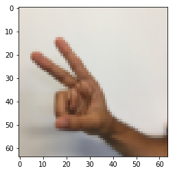
As a reminder, the SIGNS dataset is a collection of 6 signs representing numbers from 0 to 5.

The next cell will show you an example of a labelled image in the dataset. Feel free to change the value of index below and re-run to see different examples.

In [4]:

 

 

 

 

 

# Example of a picture

index = 6

plt.imshow(X_train_orig[index])

print ("y = " + str(np.squeeze(Y_train_orig[:, index])))

 

 

 

y = 2

 

 

In Course 2, you had built a fully-connected network for this dataset. But since this is an image dataset, it is more natural to apply a ConvNet to it.

To get started, let's examine the shapes of your data.

In [5]:

 

 

 

 

 

X_train = X_train_orig/255.

X_test = X_test_orig/255.

Y_train = convert_to_one_hot(Y_train_orig, 6).T

Y_test = convert_to_one_hot(Y_test_orig, 6).T

print ("number of training examples = " + str(X_train.shape[0]))

print ("number of test examples = " + str(X_test.shape[0]))

print ("X_train shape: " + str(X_train.shape))

print ("Y_train shape: " + str(Y_train.shape))

print ("X_test shape: " + str(X_test.shape))

print ("Y_test shape: " + str(Y_test.shape))

conv_layers = {}

 

 

 

number of training examples = 1080
number of test examples = 120
X_train shape: (1080, 64, 64, 3)
Y_train shape: (1080, 6)
X_test shape: (120, 64, 64, 3)
Y_test shape: (120, 6)

 

1.1 - Create placeholders

TensorFlow requires that you create placeholders for the input data that will be fed into the model when running the session.

Exercise: Implement the function below to create placeholders for the input image X and the output Y. You should not define the number of training examples for the moment. To do so, you could use "None" as the batch size, it will give you the flexibility to choose it later. Hence X should be of dimension [None, n_H0, n_W0, n_C0] and Y should be of dimension [None, n_y]. Hint.

In [6]:

 

 

 

 

 

# GRADED FUNCTION: create_placeholders

​

def create_placeholders(n_H0, n_W0, n_C0, n_y):

    """

    Creates the placeholders for the tensorflow session.

    Arguments:

    n_H0 -- scalar, height of an input image

    n_W0 -- scalar, width of an input image

    n_C0 -- scalar, number of channels of the input

    n_y -- scalar, number of classes

    Returns:

    X -- placeholder for the data input, of shape [None, n_H0, n_W0, n_C0] and dtype "float"

    Y -- placeholder for the input labels, of shape [None, n_y] and dtype "float"

    """

​

    ### START CODE HERE ### (≈2 lines)

    X = tf.placeholder(tf.float32, [None, n_H0, n_W0, n_C0])

    Y = tf.placeholder(tf.float32, [None, n_y])

    ### END CODE HERE ###

    return X, Y

 

 

In [7]:

 

 

 

 

 

X, Y = create_placeholders(64, 64, 3, 6)

print ("X = " + str(X))

print ("Y = " + str(Y))

 

 

 

X = Tensor("Placeholder:0", shape=(?, 64, 64, 3), dtype=float32)
Y = Tensor("Placeholder_1:0", shape=(?, 6), dtype=float32)

 

Expected Output

X = Tensor("Placeholder:0", shape=(?, 64, 64, 3), dtype=float32)

Y = Tensor("Placeholder_1:0", shape=(?, 6), dtype=float32)

 

1.2 - Initialize parameters

You will initialize weights/filters W1W1 and W2W2 using tf.contrib.layers.xavier_initializer(seed = 0). You don't need to worry about bias variables as you will soon see that TensorFlow functions take care of the bias. Note also that you will only initialize the weights/filters for the conv2d functions. TensorFlow initializes the layers for the fully connected part automatically. We will talk more about that later in this assignment.

Exercise: Implement initialize_parameters(). The dimensions for each group of filters are provided below. Reminder - to initialize a parameter WW of shape [1,2,3,4] in Tensorflow, use:

W = tf.get_variable("W", [1,2,3,4], initializer = ...) 

More Info.

In [16]:

 

 

 

 

 

# GRADED FUNCTION: initialize_parameters

​

def initialize_parameters():

    """

    Initializes weight parameters to build a neural network with tensorflow. The shapes are:

                        W1 : [4, 4, 3, 8]

                        W2 : [2, 2, 8, 16]

    Returns:

    parameters -- a dictionary of tensors containing W1, W2

    """

    tf.set_random_seed(1)                              # so that your "random" numbers match ours

    ### START CODE HERE ### (approx. 2 lines of code)

    W1 = tf.get_variable("W1",[4,4,3,8], initializer=tf.contrib.layers.xavier_initializer(seed=0))

    W2 = tf.get_variable("W2",[2,2,8,16], initializer=tf.contrib.layers.xavier_initializer(seed=0))

    ### END CODE HERE ###

​

    parameters = {"W1": W1,

                   "W2": W2}

    return parameters

 

 

In [17]:

 

 

 

 

 

tf.reset_default_graph()

with tf.Session() as sess_test:

    parameters = initialize_parameters()

    init = tf.global_variables_initializer()

    sess_test.run(init)

    print("W1 = " + str(parameters["W1"].eval()[1,1,1]))

    print("W2 = " + str(parameters["W2"].eval()[1,1,1]))

 

 

 

W1 = [ 0.00131723  0.14176141 -0.04434952  0.09197326  0.14984085 -0.03514394
 -0.06847463  0.05245192]
W2 = [-0.08566415  0.17750949  0.11974221  0.16773748 -0.0830943  -0.08058
 -0.00577033 -0.14643836  0.24162132 -0.05857408 -0.19055021  0.1345228
 -0.22779644 -0.1601823  -0.16117483 -0.10286498]

 

Expected Output:

W1 =	[ 0.00131723 0.14176141 -0.04434952 0.09197326 0.14984085 -0.03514394  -0.06847463 0.05245192]
W2 =	[-0.08566415 0.17750949 0.11974221 0.16773748 -0.0830943 -0.08058  -0.00577033 -0.14643836 0.24162132 -0.05857408 -0.19055021 0.1345228  -0.22779644 -0.1601823 -0.16117483 -0.10286498]

 

1.2 - Forward propagation

In TensorFlow, there are built-in functions that carry out the convolution steps for you.

• tf.nn.conv2d(X,W1, strides = [1,s,s,1], padding = 'SAME'): given an input XX and a group of filters W1W1, this function convolves W1W1's filters on X. The third input ([1,f,f,1]) represents the strides for each dimension of the input (m, n_H_prev, n_W_prev, n_C_prev). You can read the full documentation here

• tf.nn.max_pool(A, ksize = [1,f,f,1], strides = [1,s,s,1], padding = 'SAME'): given an input A, this function uses a window of size (f, f) and strides of size (s, s) to carry out max pooling over each window. You can read the full documentation here

• tf.nn.relu(Z1): computes the elementwise ReLU of Z1 (which can be any shape). You can read the full documentation here.

• tf.contrib.layers.flatten(P): given an input P, this function flattens each example into a 1D vector it while maintaining the batch-size. It returns a flattened tensor with shape [batch_size, k]. You can read the full documentation here.

• tf.contrib.layers.fully_connected(F, num_outputs): given a the flattened input F, it returns the output computed using a fully connected layer. You can read the full documentation here.

In the last function above (tf.contrib.layers.fully_connected), the fully connected layer automatically initializes weights in the graph and keeps on training them as you train the model. Hence, you did not need to initialize those weights when initializing the parameters.

Exercise:

Implement the forward_propagation function below to build the following model: CONV2D -> RELU -> MAXPOOL -> CONV2D -> RELU -> MAXPOOL -> FLATTEN -> FULLYCONNECTED. You should use the functions above.

In detail, we will use the following parameters for all the steps:

 - Conv2D: stride 1, padding is "SAME"
 - ReLU
 - Max pool: Use an 8 by 8 filter size and an 8 by 8 stride, padding is "SAME"
 - Conv2D: stride 1, padding is "SAME"
 - ReLU
 - Max pool: Use a 4 by 4 filter size and a 4 by 4 stride, padding is "SAME"
 - Flatten the previous output.
 - FULLYCONNECTED (FC) layer: Apply a fully connected layer without an non-linear activation function. Do not call the softmax here. This will result in 6 neurons in the output layer, which then get passed later to a softmax. In TensorFlow, the softmax and cost function are lumped together into a single function, which you'll call in a different function when computing the cost. 

In [10]:

 

 

 

 

 

# GRADED FUNCTION: forward_propagation

​

def forward_propagation(X, parameters):

    """

    Implements the forward propagation for the model:

    CONV2D -> RELU -> MAXPOOL -> CONV2D -> RELU -> MAXPOOL -> FLATTEN -> FULLYCONNECTED

    Arguments:

    X -- input dataset placeholder, of shape (input size, number of examples)

    parameters -- python dictionary containing your parameters "W1", "W2"

                  the shapes are given in initialize_parameters

​

    Returns:

    Z3 -- the output of the last LINEAR unit

    """

    # Retrieve the parameters from the dictionary "parameters" 

    W1 = parameters['W1']

    W2 = parameters['W2']

    ### START CODE HERE ###

    # CONV2D: stride of 1, padding 'SAME'

    Z1 = tf.nn.conv2d(X,W1,strides=[1,1,1,1],padding='SAME')

    # RELU

    A1 = tf.nn.relu(Z1)

    # MAXPOOL: window 8x8, sride 8, padding 'SAME'

    P1 = tf.nn.max_pool(A1,ksize=[1,8,8,1],strides=[1,8,8,1],padding="SAME")

    # CONV2D: filters W2, stride 1, padding 'SAME'

    Z2 = tf.nn.conv2d(P1,W2,strides=[1,1,1,1],padding='SAME')

    # RELU

    A2 = tf.nn.relu(Z2)

    # MAXPOOL: window 4x4, stride 4, padding 'SAME'

    P2 = tf.nn.max_pool(A2,ksize=[1,4,4,1],strides=[1,4,4,1],padding="SAME")

    # FLATTEN

    P2 = tf.contrib.layers.flatten(P2)

    # FULLY-CONNECTED without non-linear activation function (not not call softmax).

    # 6 neurons in output layer. Hint: one of the arguments should be "activation_fn=None" 

    Z3 = tf.contrib.layers.fully_connected(P2,6,activation_fn=None)

    ### END CODE HERE ###

​

    return Z3

 

 

In [11]:

 

 

 

 

 

tf.reset_default_graph()

​

with tf.Session() as sess:

    np.random.seed(1)

    X, Y = create_placeholders(64, 64, 3, 6)

    parameters = initialize_parameters()

    Z3 = forward_propagation(X, parameters)

    init = tf.global_variables_initializer()

    sess.run(init)

    a = sess.run(Z3, {X: np.random.randn(2,64,64,3), Y: np.random.randn(2,6)})

    print("Z3 = " + str(a))

 

 

 

Z3 = [[-0.44670227 -1.57208765 -1.53049231 -2.31013036 -1.29104376  0.46852064]
 [-0.17601591 -1.57972014 -1.4737016  -2.61672091 -1.00810647  0.5747785 ]]

 

Expected Output:

Z3 =	[[-0.44670227 -1.57208765 -1.53049231 -2.31013036 -1.29104376 0.46852064]  [-0.17601591 -1.57972014 -1.4737016 -2.61672091 -1.00810647 0.5747785 ]]

 

1.3 - Compute cost

Implement the compute cost function below. You might find these two functions helpful:

• tf.nn.softmax_cross_entropy_with_logits(logits = Z3, labels = Y): computes the softmax entropy loss. This function both computes the softmax activation function as well as the resulting loss. You can check the full documentation here.
• tf.reduce_mean: computes the mean of elements across dimensions of a tensor. Use this to sum the losses over all the examples to get the overall cost. You can check the full documentation here.

Exercise: Compute the cost below using the function above.

In [12]:

 

 

 

 

 

# GRADED FUNCTION: compute_cost 

​

def compute_cost(Z3, Y):

    """

    Computes the cost

    Arguments:

    Z3 -- output of forward propagation (output of the last LINEAR unit), of shape (6, number of examples)

    Y -- "true" labels vector placeholder, same shape as Z3

    Returns:

    cost - Tensor of the cost function

    """

    ### START CODE HERE ### (1 line of code)

    cost = tf.reduce_mean(tf.nn.softmax_cross_entropy_with_logits(logits=Z3,labels=Y))

    ### END CODE HERE ###

    return cost

 

 

In [13]:

 

 

 

 

 

tf.reset_default_graph()

​

with tf.Session() as sess:

    np.random.seed(1)

    X, Y = create_placeholders(64, 64, 3, 6)

    parameters = initialize_parameters()

    Z3 = forward_propagation(X, parameters)

    cost = compute_cost(Z3, Y)

    init = tf.global_variables_initializer()

    sess.run(init)

    a = sess.run(cost, {X: np.random.randn(4,64,64,3), Y: np.random.randn(4,6)})

    print("cost = " + str(a))

 

 

 

cost = 2.91034

 

Expected Output:

cost =

2.91034

 

1.4 Model

Finally you will merge the helper functions you implemented above to build a model. You will train it on the SIGNS dataset.

You have implemented random_mini_batches() in the Optimization programming assignment of course 2. Remember that this function returns a list of mini-batches.

Exercise: Complete the function below.

The model below should:

• create placeholders
• initialize parameters
• forward propagate
• compute the cost
• create an optimizer

Finally you will create a session and run a for loop for num_epochs, get the mini-batches, and then for each mini-batch you will optimize the function. Hint for initializing the variables

In [14]:

 

 

 

 

 

# GRADED FUNCTION: model

​

def model(X_train, Y_train, X_test, Y_test, learning_rate = 0.009,

          num_epochs = 100, minibatch_size = 64, print_cost = True):

    """

    Implements a three-layer ConvNet in Tensorflow:

    CONV2D -> RELU -> MAXPOOL -> CONV2D -> RELU -> MAXPOOL -> FLATTEN -> FULLYCONNECTED

    Arguments:

    X_train -- training set, of shape (None, 64, 64, 3)

    Y_train -- test set, of shape (None, n_y = 6)

    X_test -- training set, of shape (None, 64, 64, 3)

    Y_test -- test set, of shape (None, n_y = 6)

    learning_rate -- learning rate of the optimization

    num_epochs -- number of epochs of the optimization loop

    minibatch_size -- size of a minibatch

    print_cost -- True to print the cost every 100 epochs

    Returns:

    train_accuracy -- real number, accuracy on the train set (X_train)

    test_accuracy -- real number, testing accuracy on the test set (X_test)

    parameters -- parameters learnt by the model. They can then be used to predict.

    """

    ops.reset_default_graph()                         # to be able to rerun the model without overwriting tf variables

    tf.set_random_seed(1)                             # to keep results consistent (tensorflow seed)

    seed = 3                                          # to keep results consistent (numpy seed)

    (m, n_H0, n_W0, n_C0) = X_train.shape 

    n_y = Y_train.shape[1]                            

    costs = []                                        # To keep track of the cost

    # Create Placeholders of the correct shape

    ### START CODE HERE ### (1 line)

    X, Y = create_placeholders(n_H0, n_W0, n_C0, n_y)

    ### END CODE HERE ###

​

    # Initialize parameters

    ### START CODE HERE ### (1 line)

    parameters = initialize_parameters()

    ### END CODE HERE ###

    # Forward propagation: Build the forward propagation in the tensorflow graph

    ### START CODE HERE ### (1 line)

    Z3 = forward_propagation(X, parameters )

    ### END CODE HERE ###

    # Cost function: Add cost function to tensorflow graph

    ### START CODE HERE ### (1 line)

    cost = compute_cost(Z3, Y)

    ### END CODE HERE ###

    # Backpropagation: Define the tensorflow optimizer. Use an AdamOptimizer that minimizes the cost.

    ### START CODE HERE ### (1 line)

    optimizer = tf.train.AdamOptimizer(learning_rate=learning_rate).minimize(cost)

    ### END CODE HERE ###

    # Initialize all the variables globally

    init = tf.global_variables_initializer()

    # Start the session to compute the tensorflow graph

    with tf.Session() as sess:

        # Run the initialization

        sess.run(init)

        # Do the training loop

        for epoch in range(num_epochs):

​

            minibatch_cost = 0.

            num_minibatches = int(m / minibatch_size) # number of minibatches of size minibatch_size in the train set

            seed = seed + 1

            minibatches = random_mini_batches(X_train, Y_train, minibatch_size, seed)

​

            for minibatch in minibatches:

​

                # Select a minibatch

                (minibatch_X, minibatch_Y) = minibatch

                # IMPORTANT: The line that runs the graph on a minibatch.

                # Run the session to execute the optimizer and the cost, the feedict should contain a minibatch for (X,Y).

                ### START CODE HERE ### (1 line)

                _ , temp_cost = sess.run([optimizer,cost],feed_dict={X:minibatch_X, Y:minibatch_Y})

                ### END CODE HERE ###

                minibatch_cost += temp_cost / num_minibatches

​

            # Print the cost every epoch

            if print_cost == True and epoch % 5 == 0:

                print ("Cost after epoch %i: %f" % (epoch, minibatch_cost))

            if print_cost == True and epoch % 1 == 0:

                costs.append(minibatch_cost)

        # plot the cost

        plt.plot(np.squeeze(costs))

        plt.ylabel('cost')

        plt.xlabel('iterations (per tens)')

        plt.title("Learning rate =" + str(learning_rate))

        plt.show()

​

        # Calculate the correct predictions

        predict_op = tf.argmax(Z3, 1)

        correct_prediction = tf.equal(predict_op, tf.argmax(Y, 1))

        # Calculate accuracy on the test set

        accuracy = tf.reduce_mean(tf.cast(correct_prediction, "float"))

        print(accuracy)

        train_accuracy = accuracy.eval({X: X_train, Y: Y_train})

        test_accuracy = accuracy.eval({X: X_test, Y: Y_test})

        print("Train Accuracy:", train_accuracy)

        print("Test Accuracy:", test_accuracy)

        return train_accuracy, test_accuracy, parameters

 

 

 

Run the following cell to train your model for 100 epochs. Check if your cost after epoch 0 and 5 matches our output. If not, stop the cell and go back to your code!

In [15]:

 

 

 

 

 

_, _, parameters = model(X_train, Y_train, X_test, Y_test)

 

 

 

Cost after epoch 0: 1.917929
Cost after epoch 5: 1.506757
Cost after epoch 10: 0.955359
Cost after epoch 15: 0.845802
Cost after epoch 20: 0.701174
Cost after epoch 25: 0.571977
Cost after epoch 30: 0.518435
Cost after epoch 35: 0.495806
Cost after epoch 40: 0.429827
Cost after epoch 45: 0.407291
Cost after epoch 50: 0.366394
Cost after epoch 55: 0.376922
Cost after epoch 60: 0.299491
Cost after epoch 65: 0.338870
Cost after epoch 70: 0.316400
Cost after epoch 75: 0.310413
Cost after epoch 80: 0.249549
Cost after epoch 85: 0.243457
Cost after epoch 90: 0.200031
Cost after epoch 95: 0.175452

 

 

Tensor("Mean_1:0", shape=(), dtype=float32)
Train Accuracy: 0.940741
Test Accuracy: 0.783333

 

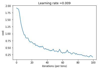
Expected output: although it may not match perfectly, your expected output should be close to ours and your cost value should decrease.

Cost after epoch 0 =	1.917929
Cost after epoch 5 =	1.506757
Train Accuracy =	0.940741
Test Accuracy =	0.783333

 

Congratulations! You have finised the assignment and built a model that recognizes SIGN language with almost 80% accuracy on the test set. If you wish, feel free to play around with this dataset further. You can actually improve its accuracy by spending more time tuning the hyperparameters, or using regularization (as this model clearly has a high variance).

Once again, here's a thumbs up for your work!

转载于:https://www.cnblogs.com/Dar-/p/9527845.html