The most beautiful graph you have ever seen, courtesy of https://www.quora.com/Whats-the-most-beautiful-graph-you-have-ever-seen.
In this article, I will walk you through the details of text-based Graph Convolutional Network (GCN) and its implementation using PyTorch and standard libraries. The text-based GCN model is an interesting and novel state-of-the-art semi-supervised learning concept that was proposed recently(expanding upon the previous GCN idea by Kipf et al. on non-textual data) which is able to very accurately infer the labels of some unknown textual data given related known labeled textual data.
At the highest level, it does so by embedding the entire corpus into a single graph with documents (some labelled and some unlabelled) and words as nodes, with each document-word & word-word edges having some predetermined weights based on their relationships with each other (eg. Tf-idf). A GCN is then trained on this graph with documents nodes that have known labels, and the trained GCN model is then used to infer the labels of unlabelled documents.
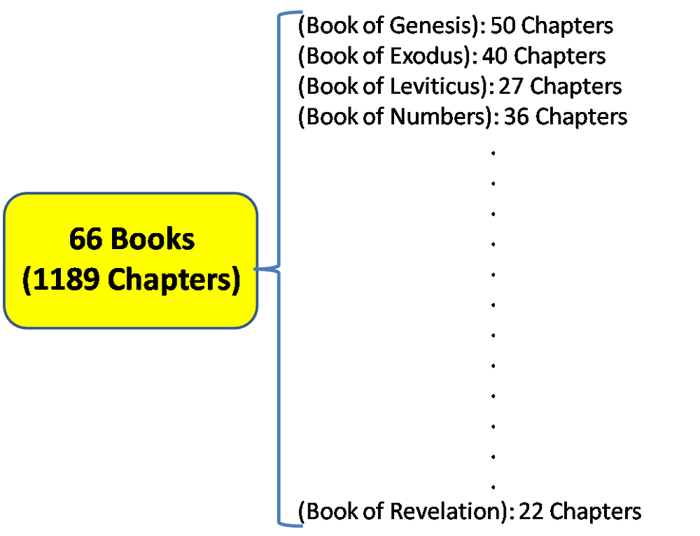
We implement text-based GCN here using the Holy Bible as the corpus, which is chosen because it is one of the most read book in the world and contains a rich structure of text. The Holy Bible (Protestant) consists of 66 Books (Genesis, Exodus, etc) and 1189 Chapters. The semi-supervised task here is to train a language model that is able to correctly classify the Book that some unlabelled Chapters belong to, given the known labels of other Chapters. (Since we actually do know the exact labels of all Chapters, we will intentionally mask the labels of some 10–20 % of the Chapters, which will be used as test set during model inference to measure the model accuracy)
Structure of the Holy Bible (Protestant)
To solve this task, the language model needs to be able to distinguish between the contexts associated with the various Books (eg. Book of Genesis talks more about Adam & Eve while the Book of Ecclesiastes talks about the life of King Solomon). The obtained good results of the text-GCN model, as we shall see below, show that the graph structure is able to capture such context relatively well, where the document (Chapter)-word edges encode the context within Chapters, while the word-word edges encode the relative context between Chapters.
The Bible text used here (BBE version) is obtained courtesy of https://github.com/scrollmapper/bible_databases.
Implementation follows the paper on Text-based Graph Convolutional Network (https://arxiv.org/abs/1809.05679)
The source codes for the implementation can be found in my GitHub repository (https://github.com/plkmo/Bible_Text_GCN)
Representing the Corpus
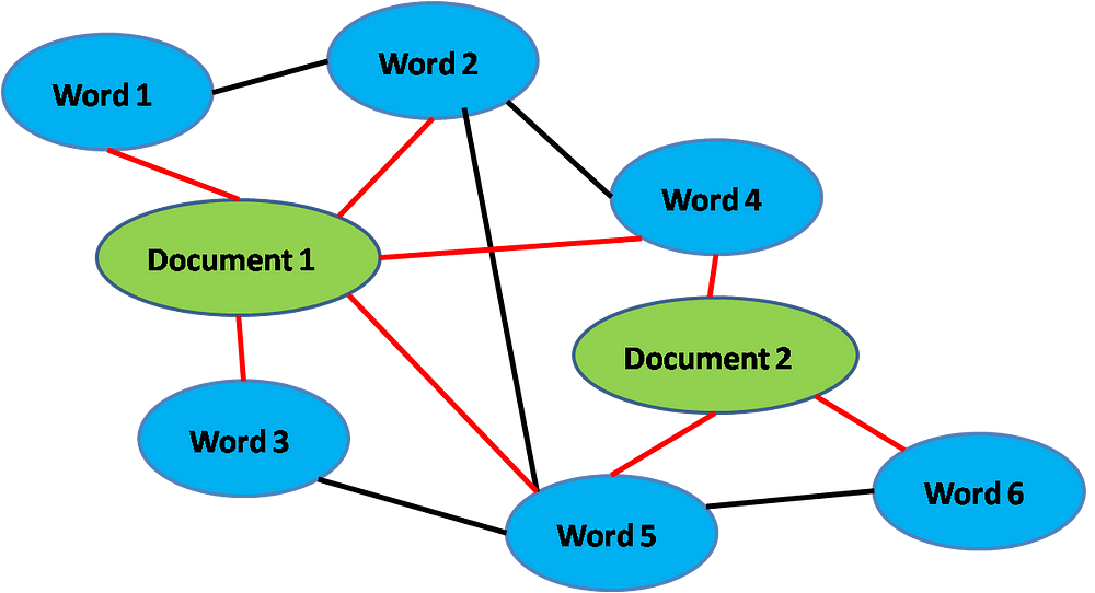
Corpus represented as a graph. Red lines represent document-word edges weighted by TF-IDF, black lines represent word-word edges weighted by PMI.
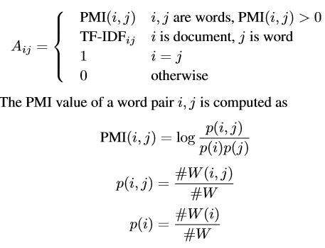
Following the paper, in order to allow GCN to capture the Chapter contexts, we build a graph with nodes and edges that represent the relationships between Chapters and words. The nodes will consist of all 1189 Chapters (documents) plus the whole vocabulary (words), with weighted document-word and word-word edges between them. Their weights A_ij are given by:
Edges weights
where PMI is the Point-wise Mutual Information between pairs of co-occurring words over a sliding window #W that we fix to be of 10-words length. #W(i) is the number of sliding windows in a corpus that contain word i, #W(i,j) is the number of sliding windows that contain both word i and j, and #W is the total number of sliding windows in the corpus. TF-IDF is the usual term frequency-inverse document frequency of the word in the document. Intuitively, a high positive PMI between pairs of words means that they have a high semantic correlation, conversely we do not build edges between words with negative PMI. Overall, TF-IDF-weighted document-word edges capture within-document context, while PMI-weighted word-word edges (which can span across documents) capture across-document contexts.
In comparison, for non-graph based models, such across-document context information are not easily provided as input features, and the model would have to learn them by itself “from scratch” based on the labels. Since additional information on the relationship between documents is provided in GCN which is definitely relevant in NLP tasks, one would expect that GCN would perform better.
- Calculating TF-IDF
### Tfidf
vectorizer = TfidfVectorizer(input="content", max_features=None, tokenizer=dummy_fun, preprocessor=dummy_fun)
vectorizer.fit(df_data["c"])
df_tfidf = vectorizer.transform(df_data["c"])
df_tfidf = df_tfidf.toarray()
vocab = vectorizer.get_feature_names()
vocab = np.array(vocab)
df_tfidf = pd.DataFrame(df_tfidf,columns=vocab)
Calculating TF-IDF is relatively straightforward. We know the math and understand how it works, so we simply use sklearn’s TfidfVectorizer module on our 1189 documents texts, and store the result in a dataframe. This will be used for the document-word weights when we create the graph later.
2. Calculating Point-wise Mutual Information between words
### PMI between words
window = 10 # sliding window size to calculate point-wise mutual information between words
names = vocab
occurrences = OrderedDict((name, OrderedDict((name, 0) for name in names)) for name in names)
# Find the co-occurrences:
no_windows = 0; print("calculating co-occurences")
for l in df_data["c"]:
    for i in range(len(l)-window):
        no_windows += 1
        d = l[i:(i+window)]; dum = []
        for x in range(len(d)):
            for item in d[:x] + d[(x+1):]:
                if item not in dum:
                    occurrences[d[x]][item] += 1; dum.append(item)

df_occurences = pd.DataFrame(occurrences, columns=occurrences.keys())
df_occurences = (df_occurences + df_occurences.transpose())/2 ## symmetrize it as window size on both sides may not be same
del occurrences
### convert to PMI
p_i = df_occurences.sum(axis=0)/no_windows
p_ij = df_occurences/no_windows
del df_occurences
for col in p_ij.columns:
    p_ij[col] = p_ij[col]/p_i[col]
for row in p_ij.index:
    p_ij.loc[row,:] = p_ij.loc[row,:]/p_i[row]
p_ij = p_ij + 1E-9
for col in p_ij.columns:
    p_ij[col] = p_ij[col].apply(lambda x: math.log(x))
Calculating PMI between words is more tricky. First, we need to find the co-occurrences between words i, j within a sliding window of 10 words, stored as a square matrix in a dataframe where rows and columns represent the vocabulary. From this, we can then calculate the PMI using the definition earlier. The annotated code for the calculation is shown above.
3. Build the graph
Now that we have all the weights for the edges, we are ready to build the graph G. We use the networkx module to build it. Here, its noteworthy to point out that most of the heavy-lifting computation for this whole project is spent on building the word-word edges, as we need to iterate over all possible pairwise word combinations for a vocabulary of about 6500 words. In fact, a full 2 days is spent computing this. The code snippet for our computation is shown below.
def word_word_edges(p_ij):
    dum = []; word_word = []; counter = 0
    cols = list(p_ij.columns); cols = [str(w) for w in cols]
    for w1 in cols:
        for w2 in cols:
            if (counter % 300000) == 0:
                print("Current Count: %d; %s %s" % (counter, w1, w2))
            if (w1 != w2) and ((w1,w2) not in dum) and (p_ij.loc[w1,w2] > 0):
                word_word.append((w1,w2,{"weight":p_ij.loc[w1,w2]})); dum.append((w2,w1))
            counter += 1
    return word_word

### Build graph
G = nx.Graph()
G.add_nodes_from(df_tfidf.index) ## document nodes
G.add_nodes_from(vocab) ## word nodes
### build edges between document-word pairs
document_word = [(doc,w,{"weight":df_tfidf.loc[doc,w]}) for doc in df_tfidf.index for w in df_tfidf.columns]
G.add_edges_from(document_word)
### build edges between word-word pairs
word_word = word_word_edges(p_ij)
G.add_edges_from(word_word)
Graph Convolutional Network
In convolutional neural networks for image-related tasks, we have convolution layers or filters (with learnable weights) that “pass over” a bunch of pixels to generate feature maps that are learned by training. Now imagine that these bunch of pixels are your graph nodes, we will similarly have a bunch of filters with learnable weights W that “pass over” these graph nodes in GCN.
However, there is a big problem: graph nodes do not really have a clear notion of physical space and distance as pixels have (we can’t really say that a node is to the right or left of another). As such, in order to meaningfully convolve nodes with our filter W, we have to first find feature representations for each node that best captures the graph structure. For the advanced readers, the authors solved this problem by projecting both the filter weights W and feature space X for each node into the Fourier space of the graph, so that convolution becomes just a point-wise multiplication of nodes with features. For a deep dive into the derivation, the original paper by Kipf et al. is a good starting point. Otherwise, the readers can just make do with this intuitive explanation and proceed on.
We are going to use a two-layer GCN (features are convolved twice) here as, according to their paper, it gives the best results. The convoluted output feature tensor after the two-layer GCN is given by:
where
Here, A is the adjacency matrix of graph G (with diagonal elements being 1 to represent self-connection of nodes) and D is the degree matrix ofG. W_0 and W_1 are the learnable filter weights for the first and second GCN layer respectively, which is to be trained. X is the input feature matrix which we take to be a diagonal square matrix (of ones) of the same dimension as the number of nodes, which simply means that the input is a one-hot encoding of each of the graph nodes. The final output is then fed into a softmax layer with a cross entropy loss function for classification with 66 different labels corresponding to each of the 66 books.
The implementation of the two-layer GCN architecture in PyTorch is given below.
### GCN architecture, with Xavier’s initialization of W_0 (self.weight) and W_1(self.weight2) as well as biases.
class gcn(nn.Module):
    def __init__(self, X_size, A_hat, bias=True): # X_size = num features
        super(gcn, self).__init__()
        self.A_hat = torch.tensor(A_hat, requires_grad=False).float()
        self.weight = nn.parameter.Parameter(torch.FloatTensor(X_size, 330))
        var = 2./(self.weight.size(1)+self.weight.size(0))
        self.weight.data.normal_(0,var)
        self.weight2 = nn.parameter.Parameter(torch.FloatTensor(330, 130))
        var2 = 2./(self.weight2.size(1)+self.weight2.size(0))
        self.weight2.data.normal_(0,var2)
        if bias:
            self.bias = nn.parameter.Parameter(torch.FloatTensor(330))
            self.bias.data.normal_(0,var)
            self.bias2 = nn.parameter.Parameter(torch.FloatTensor(130))
            self.bias2.data.normal_(0,var2)
        else:
            self.register_parameter("bias", None)
        self.fc1 = nn.Linear(130,66)

    def forward(self, X): ### 2-layer GCN architecture
        X = torch.mm(X, self.weight)
        if self.bias is not None:
            X = (X + self.bias)
        X = F.relu(torch.mm(self.A_hat, X))
        X = torch.mm(X, self.weight2)
        if self.bias2 is not None:
            X = (X + self.bias2)
        X = F.relu(torch.mm(self.A_hat, X))
        return self.fc1(X)
Training Phase
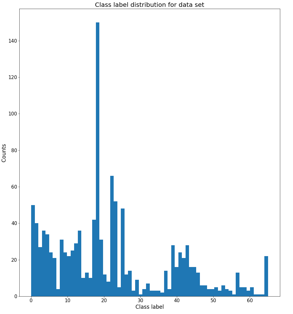
Class label distribution
Out of a total of 1189 Chapters, we will mask the labels of 111 of them (about 10 %) during training. As the class label distribution over 1189 Chapters are quite skewed (above figure), we will not mask any of the class labels of those Chapters in which their total count is less than 4, to ensure that the GCN can learn representations from all 66 unique class labels.
We train the GCN model to minimize the cross entropy losses of the unmasked labels. After training the GCN for 7000 epochs, we will then use the model to infer the Book labels of the 111 masked Chapters and analyze the results.
Results
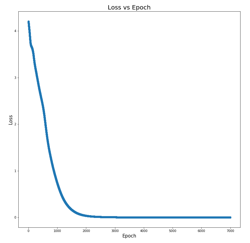
Loss vs Epoch
From the Loss vs Epoch graph above, we see that training proceeds pretty well and starts to saturate at around 2000 epochs.
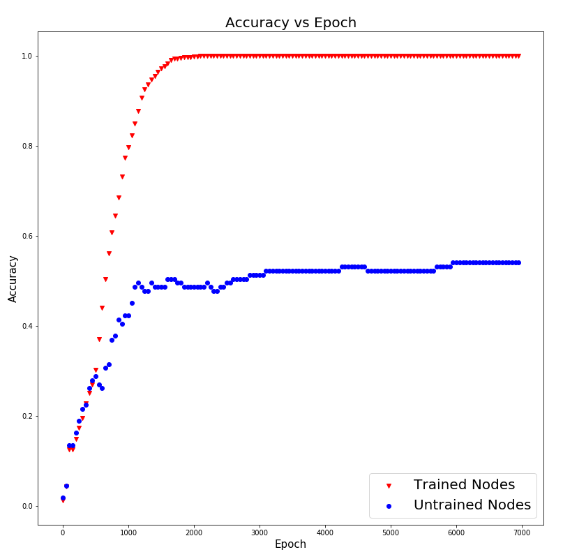
Accuracy of training nodes (trained nodes) and inference accuracy of masked nodes (untrained nodes) with epoch.
As training proceeds, the training accuracy as well as the inference accuracy (of the masked nodes) are seen to increase together, until about 2000 epochs where the inference accuracy starts to saturate at around 50%. Considering that we have 66 classes, which would have a baseline accuracy of 1.5 % if we assume that the model predicts by pure chance, thus 50% inference accuracy seems pretty good already. This tells us that the GCN model is able to correctly infer the Book which the given unlabelled Chapter belongs to about 50 % of the time, after being trained properly on labelled Chapters.
Misclassified Chapters
The GCN model is able to capture the within-document and between-document contexts pretty well, but what about the misclassified Chapters? Does it mean that the GCN model failed on those? Lets look at a few of them to find out.
- Book: Matthew
Chapter 27: “Now when it was morning, all the chief priests and those in authority took thought together with the purpose of putting Jesus to death. And they put cords on Him and took Him away, and gave Him up to Pilate, the ruler. Then Judas, who was false to Him, seeing that He was to be put to death, in his regret took back the thirty bits of silver to the chief priests and those in authority, saying, I have done wrong in giving into your hands an upright man. But they said, what is that to us? It is your business. and he put down the silver in the temple and went out, and put himself to death by hanging. And the chief priests took the silver and said, it is not right to put it in the temple store for it is the price of blood. And they made a decision to get with the silver the potter’s field, as a place for the dead of other countries. For this cause that field was named…He has come back from the dead: and the last error will be worse than the first. Pilate said to them, you have watchmen; go and make it as safe as you are able. So they went, and made safe the place where His body was, putting a stamp on the stone, and the watchmen were with them.”
Predicted as: Luke
In this case, Chapter 27 from the book of Matthew has been wrongly classified to be from the book of Luke. From above, we see that this Chapter is about Jesus being put to death by the chief priests and dying for our sins, as well as Judas’s guilt after his betrayal of Jesus. Now, these events are also mentioned in Luke! (as well as in Mark and John) This is most likely why the model classified it as Luke, as they share similar context.
- Book: Isaiah
Chapter 12: “And in that day you will say I will give praise to you, O Lord; For though You were angry with me, Your wrath is turned away, and I am comforted. See, God is my salvation; I will have faith in the Lord, without fear: For the Lord is my strength and song; and He has become my salvation. So with joy will you get water out of the springs of salvation. And in that day you will say, give praise to the Lord, let His name be honored, give word of His doings among the peoples, say that His name is lifted up. Make a song to the Lord; for He has done noble things: give news of them through all the earth. Let your voice be sounding in a cry of joy, O daughter of Zion, for great is the Holy One of Israel among you.”
Predicted as Psalms
Here, Chapter 12 from the Book of Isaiah is wrongly inferred to be from the Book of Psalms. It is clear from this passage that the narrator in Isaiah Chapter 12 talks about giving and singing praises to God, who is his comforter and source of salvation. This context of praising God and looking to Him for comfort is exactly the whole theme of the Book of Psalms, where David pens down his praises and prayers to God throughout his successes, trials and tribulations! Hence, it is no wonder that the model would classify it as Psalms, as they share similar context.
Conclusion
The text-based Graph Convolutional Network is indeed a powerful model especially for semi-supervised learning, as it is able to strongly capture the textual context between and across words and documents, and infer the unknown given the known.
The applications of GCNs are actually quite robust and far-reaching, and this article has only provided a glimpse of what it can do. In general other than for the task presented here, GCN can be used whenever one wants to combine the power of graph representations with deep learning. To provide a few interesting examples for further reading, GCN has been used in combination with Recurrent Neural Networks (RNNs)/Long Short-Term Memory (LSTMs)for dynamic network/node/edge predictions. It has also been successfully applied for dynamic pose estimation of the human skeleton by modelling human joints as graph nodes and the relationships between and within human body structures and time-frames as graph edges.
Thanks for reading and I hope that this article has helped much to explain its inner workings.
References
- Thomas N. Kipf, Max Welling, Semi-Supervised Classification with Graph Convolutional Networks (https://arxiv.org/abs/1609.02907) (2016)
- Liang Yao, Chengsheng Mao, Yuan Luo, Graph Convolutional Networks for Text Classification (https://arxiv.org/abs/1809.05679) (2018)
This article is first published in
https://towardsdatascience.com/text-based-graph-convolutional-network-for-semi-supervised-bible-book-classification-c71f6f61ff0f







 1034
1034

 被折叠的 条评论
为什么被折叠?


