Causal Inference: Trying to Understand the Question of Why

Why are you reading this article? Why did you choose to learn about causal inference? Why are you thinking that this is a really weird way to start an article? Who knows. A more interesting question to ask is why can we, as humans, think about and understand the question “why” in the first place!? If we ever want to create a system with Artificial General Intelligence, or AGI, we need to answer this question.

 

understanding why requires understanding of the whats, the wheres, and the whens. The hows, however, seem to be an implementation of the whys. image source.

You, and everyone else on this planet, are able to understand cause-and-effect relationships, an ability that is still largely lacking in machines. And before we can think about creating a system that can generally understand cause-and-effect, we should look at cause-and-effect from a statistics perspective: causal calculus and causal inference. Statistics is where causality was born from, and in order to create a high-level causal system, we must return to the fundamentals.

Causal Inference is the process where causes are inferred from data. Any kind of data, as long as have enough of it. (Yes, even observational data). It sounds pretty simple, but it can get complicated. We, as humans, do this everyday, and we navigate the world with the knowledge we learn from causal inference. And not only do we use causal inference to navigate the world, we use causal inference to solve problems.

 

15 million premature babies are born every year. image source.

Every year, 1.1 million premature babies die. In other words, 7.3% of all premature babies die every single year. Millions of parents have to struggle through the grief, suffering, and pain of losing their child over a process they can’t control. That’s a problem. Let’s say we want to figure out whether comprehensive treatment after the birth of a premature baby will affect its chances for survival. In order to solve this problem, we need to use causal inference.

The python library we’ll be using to perform causal inference to solve this problem is called DoWhy, a well-documented library created by researchers from Microsoft.

 

A Quick Lesson on Causality

First, a quick lesson on causality (if you already know the basics, you can skip this section; if you prefer to watch a video, lucky you, I made one that you can watch here).

Causality is all about interventions, about doing. Standard statistics is all about correlations, which are all good and fun, but correlations can lead to wrong assumptions which can lead to a lot worse things.

 

This is a graph showing the correlative relationship between Exercise and Cholesterol (which looks like a causal relationship but is not). If we just look at the correlative relationship between cholesterol and exercise, it looks like there’s a causal relationship between the two. But this correlation actually happens because both cholesterol and exercise share a common cause or confounder: age. image source.

In correlations, the notation is P(x|y) i.e. the probability of x given y: for example, the probability of a disease given an active gene. However, in causal calculus, a very small but important change is made. Instead of P(x|y) it’s P(x|do(y)) i.e. the probability of x given that y is done: for example, the probability of a disease given that I start a diet. The ‘do’ is very important: it represents the intervention, the actual doing of something that will cause the effect.

If this ‘do’ stuff still isn’t making too much sense, let me take you through another example:

Take air-pressure and a barometer. There is a correlation between the reading on a barometer and the air-pressure, but, in a standard correlation (P(x|y)) we wouldn’t be able to tell which one caused which. However if we switched it up to causal calculus, otherwise known as do-calculus (yes, the ‘do’ is everywhere) we could ask a question like, “What is the probability of a high barometer reading given that the pressure increases?” Increasing the pressure is the act of doing, and through doing and intervening, we can see if there is a clear causal relationship between the two variables. (Clearly we would see an increase in the barometer reading if we increased the pressure).

This works vice-versa as well. If we changed the reading on the barometer (by twisting a knob or something, which is an act of doing) we would not see the air-pressure change because the barometer reading does not cause the air-pressure. The air-pressure affects the barometer reading.

 

air pressure -> barometer reading. source.

However, the air pressure and barometer example is pretty simple; there are only two factors. In real life, there are countless factors that each have some sort of causal relationship with the others.

 

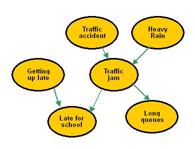
an example of a causal diagram. image source.

In the diagram, “traffic jam” is a confounder or common cause for “late for school” and “long queues”. Confounders are variables that have a causal relationship with two variables that we want to test a causal relationship between. If we wanted to test the causal relationship between “late for school” and “long queues”, we would have to account for “traffic jam” in order to make sure of the validity of the causal relationship found between “late for school” and “long queues”, as in the cholesterol example of above. In causal inference, we always need to account for confounders because they introduce correlations that muddle the causal diagram.

IHDP Dataset

Ok now that we have a good understanding of basic causality, let’s actually get to the code and test the causal relationship between the wellbeing of a premature twin and intervention. We’ll be using the dataset from the Infant Health and Development Program (IHDP) which collected data on premature infants in randomized trials in the US from 1985–1988. Randomization is key because it provides an unbiased account of the world. Because this data was collected in an RCT, causal inference is not necessary, but we will still do it to show how it works.

An intensive intervention extending from hospital discharge to 36 months corrected age was administered between 1985 and 1988 at eight different sites. The study sample of infants was stratified by birth weight (2,000 grams or less, 2,001–2,500 grams) and randomized to the Intervention Group or the Follow-Up Group. The Intervention Group received home visits, attendance at a special child development center, and pediatric follow-up. The Follow-Up Group received only the pediatric follow-up component of the program. Measures of cognitive development, behavioral status, health status, and other variables were collected from both groups at predetermined time points…. The many other variables and indices in the data collection include site, pregnancy complications, child’s birth weight and gestation age, birth order, child’s gender, household composition, day care arrangements, source of health care, quality of the home environment, parents’ race and ethnicity, and maternal age, education, IQ, and employment. — from the HMCA archive.

The Code

First, let’s import the required package and load the data.

import dowhy
from dowhy import CausalModel
import pandas as pd
import numpy as npdata= pd.read_csv(“https://raw.githubusercontent.com/AMLab-Amsterdam/CEVAE/master/datasets/IHDP/csv/ihdp_npci_1.csv", header = None)col = [“treatment”, “y_factual”, “y_cfactual”, “mu0”, “mu1” ,]for i in range(1,26):
 col.append(“x”+str(i))data.columns = col
data = data.astype({“treatment”:’bool’}, copy=False)
print(data.head())
____________________________________________________________________  treatment y_factual y_cfactual mu0      … x22 x23 x24 x250 True      5.599916 4.318780    3.268256 … 0   0   0   01 False     6.875856 7.856495    6.636059 … 0   0   0   02 False     2.996273 6.633952    1.570536 … 0   0   0   03 False     1.366206 5.697239    1.244738 … 0   0   0   04 False     1.963538 6.202582    1.685048 … 0   0   0   0

Treatment here is the intervention. Y_factual is the outcome, quantified through the combination of the mental, behavioral, and health statuses of the infants. All the x’s (x1 to x25) are confounders of the outcome and the intervention: variables like gender, race, quality of home-care, etc. We’re trying to figure out the causal relationship between the treatment and the outcome, while accounting for the confounders. (Technically we don’t have to account for these confounders because the data was collected through a randomized trial and any bias that would build up with them would be wiped out. However, it’s still a good idea to account for them, and it’s absolutely necessary to account for them when the data is observational).

We don’t care about y_cfactual, mu0, and mu1 (they’re used by the creators of the GitHub linked in the code (a super cool project on a Causal Effect Variational AutoEncoder, or CEVAE, that you should totally check out))

If you’re interested in what they are:

y_cfactual is a counterfactual, which is a question about something that didn’t happen, like “What would happen if I…?” In this case, it's a prediction as to what would happen if there was, or was not, an intervention (depending on the context). Counterfactuals are extremely important in causality because most of the times we aren’t always able to get all the data. For example, if we wanted to test the effectiveness of two different treatments on a single person, we would not be able to test both of them. Counterfactuals address the “imaginary” treatment that did not actually get administered, and we, as humans, use counterfactuals all the time (every time you imagine an alternate situation). If you’re more interested about them, read this great blog post here.

Mu0 and mu1 are conditional means, in other words the expected or average value of y_factual with and without a treatment. The creators of the GitHub used these variables (y_cfactual, mu0, and mu1) to test the strength of the CEVAE.

Ok so now we have all the data setup, organized in a way that is convenient for causal inference. It’s time to actually do causal inference.

Causal Inference with DoWhy!

DoWhy breaks down causal inference into four simple steps: model, identify, estimate, and refute. We’ll follow these steps as we perform causal inference.

Model

# Create a causal model from the data and given common causes.
xs = ""
for i in range(1,26):
    xs += ("x"+str(i)+"+")model=CausalModel(
        data = data,
        treatment='treatment',
        outcome='y_factual',
        common_causes=xs.split('+')
        )

This code actually takes the data and makes a causal model, or causal diagram, with it.

 

the (visually unpleasant) graph created by DoWhy of the causal model

Even though we aren’t printing anything out, DoWhy will still give us warnings and information updates about our causal inference (which is super nice for beginners). In this case, it gives us:

WARNING:dowhy.causal_model:Causal Graph not provided. DoWhy will construct a graph based on data inputs.
INFO:dowhy.causal_model:Model to find the causal effect of treatment ['treatment'] on outcome ['y_factual']

Identify

#Identify the causal effect
identified_estimand = model.identify_effect()
print(identified_estimand)

The identify step uses the causal diagram created from the model step and identifies all the causal relationships. This code prints out:

INFO:dowhy.causal_identifier:Common causes of treatment and outcome:['', 'x6', 'x3', 'x14', 'x10', 'x16', 'x9', 'x17', 'x13', 'x4', 'x11', 'x1', 'x7', 'x24', 'x25', 'x20', 'x5', 'x21', 'x2', 'x19', 'x23', 'x8', 'x15', 'x18', 'x22', 'x12']WARNING:dowhy.causal_identifier:If this is observed data (not from a randomized experiment), there might always be missing confounders. Causal effect cannot be identified perfectly.WARN: Do you want to continue by ignoring any unobserved confounders? (use proceed_when_unidentifiable=True to disable this prompt) [y/n] yINFO:dowhy.causal_identifier:Instrumental variables for treatment and outcome:[]Estimand type: nonparametric-ate### Estimand : 1Estimand name: backdoorEstimand expression:d(Expectation(y_factual|x6,x3,x14,x10,x16,x9,x17,x13,x4,x11,x1,x7,x24,x25,x20,x5,x21,x2,x19,x23,x8,x15,x18,x22,x12)) / d[treatment]Estimand assumption 1, Unconfoundedness: If U→{treatment} and U→y_factual then P(y_factual|treatment,x6,x3,x14,x10,x16,x9,x17,x13,x4,x11,x1,x7,x24,x25,x20,x5,x21,x2,x19,x23,x8,x15,x18,x22,x12,U) = P(y_factual|treatment,x6,x3,x14,x10,x16,x9,x17,x13,x4,x11,x1,x7,x24,x25,x20,x5,x21,x2,x19,x23,x8,x15,x18,x22,x12)### Estimand : 2Estimand name: ivNo such variable found!

Since we’re not trying to find 2 causal relationships (just trying to find the effect of intervention on outcome) estimand 2 is not found.

Estimate

Using the estimand (the causal relationship identified) we can now estimate the strength of this causal relationship. There are many methods available to us (propensity-based-matching, additive noise modeling), but in this tutorial, we’ll stick to good ol’ fashioned linear regression.

# Estimate the causal effect and compare it with Average Treatment Effectestimate = model.estimate_effect(identified_estimand, method_name="backdoor.linear_regression", test_significance=True)print(estimate)print("Causal Estimate is " + str(estimate.value))data_1 = data[data["treatment"]==1]
data_0 = data[data["treatment"]==0]
print("ATE", np.mean(data_1["y_factual"])- np.mean(data_0["y_factual"]))

Using linear regression, the model trains on the cause (the intervention) and the effect (the wellbeing of the premature baby) and identifies the strength in the relationship between the two. I also printed out the ATE (Average Treatment Effect (the difference between the averages of the group that received treatment from the group that didn’t)) The ATE is a good indicator/number we can check out causal effect with, in this case, because the data was retrieved in randomized trials instead of from observational data. Observational data would have unobserved confounders (factors that affect both the treatment and the outcome) or instrumental variables (factors that only affect the treatment and are thus correlated with the outcome) that ATE would not be able to account for. ATE is not the same as the causal effect found through linear regression because it does not account for confounders.

INFO:dowhy.causal_estimator:INFO: Using Linear Regression EstimatorINFO:dowhy.causal_estimator:b: y_factual~treatment+x6+x3+x14+x10+x16+x9+x17+x13+x4+x11+x1+x7+x24+x25+x20+x5+x21+x2+x19+x23+x8+x15+x18+x22+x12*** Causal Estimate ***--prints out the estimand again––## Realized estimandb:y_factual~treatment+x6+x3+x14+x10+x16+x9+x17+x13+x4+x11+x1+x7+x24+x25+x20+x5+x21+x2+x19+x23+x8+x15+x18+x22+x12## EstimateValue: 3.928671750872714## Statistical Significancep-value: <0.001Causal Estimate is 3.928671750872714ATE 4.021121012430832

As you can see, the ATE is pretty close to the Causal Estimate that we got. The ~4 is the difference in wellbeing of the premature babies that had care vs. those who didn’t. The number 4 doesn’t have much meaning semantically because it is the literal difference of the outcome between the two groups, and the outcome, in this case, was a combination of a variety of other factors. If you take a look back at the 5 cases that were printed out, the differences between the two are about 4.

Refute

The refute steps tests the strength and validity of the causal effect found by the estimate step. There are a variety of different refutation methods, eg. Subset Validation (using only a subset of the data to estimate the causal effect) or Placebo Treatment (turning the treatment into a placebo and seeing its effect on the outcome (the placebo treatment refutation expects the causal effect to go down)) In this case, we’ll be adding an irrelevant common cause to test the strength of the causal relationship between the treatment and outcome. This is useful because it changes the causal model but not the relationship between y_factual and treatment.

refute_results=model.refute_estimate(identified_estimand, estimate,
        method_name="random_common_cause")
print(refute_results)
____________________________________________________________________INFO:dowhy.causal_estimator:INFO: Using Linear Regression EstimatorINFO:dowhy.causal_estimator:b: y_factual~treatment+x22+x4+x24+x7+x20+x19+x21+x1+x23+x2+x12+x18+x3+x10+x14+x11+x16+x9+x13+x5+x17+x15+x6+x8+x25+w_randomRefute: Add a Random Common CauseEstimated effect:(3.928671750872715,)New effect:(3.9280606136724203,)

Adding a random common cause didn’t have much of an effect on the causal effect (as expected) and so we can be more assured of the strength of the causal relationship.

OK, so we just found out that there is a clear causal relationship between intervention on premature babies and their wellbeing using causal inference with DoWhy. In the future, instead of performing causal inference in narrow examples like this, we want a system that can understand causal relationships generally without much data. Right now, we still don’t even understand how the brain understands cause-and-effect, but now that we understand how to perform causal inference from a statistical perspective, we are much better prepared to tackle that problem. To create Artificial General Intelligence, causality needs to be understood and implemented generally, and I hope to work on such a project in the near future!