Deep learning 吴恩达 course-1

Week 1

• 对于图像应用，我们经常在神经网络上使用卷积（Convolutional Neural Network），通常缩写为CNN。对于序列数据，例如音频，有一个时间组件，随着时间的推移，音频被播放出来，所以音频是最自然的表现。作为一维时间序列（两种英文说法one-dimensional time series / temporal sequence）.对于序列数据，经常使用RNN，一种递归神经网络（Recurrent Neural Network），语言，英语和汉语字母表或单词都是逐个出现的，所以语言也是最自然的序列数据，因此更复杂的RNNs版本经常用于这些应用。
• structured data ：dataset
  unstructured data：image，voice

Week 2

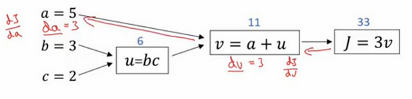
forward/backward propagation 前向/反向 传播

n = dimension of input feature victor
m = training examples

我们用parameter w来表示逻辑回归的参数，这也是一个nx维向量（因为实际上是特征权重，维度与特征向量相同），参数里面还有b，这是一个实数（表示偏差）。
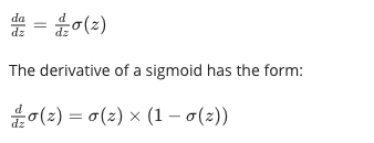
sigmoid函数的公式是这样的，Z在这里是一个实数

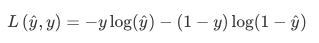
• Loss（error） function：我们称为损失函数，来衡量预测输出值和实际值有多接近。
  
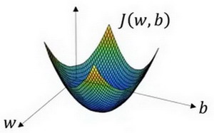
• Cost function ：损失函数只适用于单个训练样本，而cost function是用于衡量the entire training set
  

local / global optima 局部/全局最优解
optimize 优化

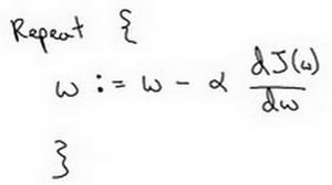
梯度下降法 gradient decent

derivative 导数
slope 斜率

变量命名

dvar：最终的输出变量，你真正想要关心或者说优化的。

逻辑回归中的梯度下降（Logistic Regression Gradient Descent）

$$da=\frac{\partial L}{\partial a}=-\frac{y}{a}+\frac{1-y}{1-a}$$
$$\frac{\partial a}{\partial z}=a(1-a)$$
$$dz=\frac{\partial L}{\partial z}=\frac{\partial L}{\partial a}\ast \frac{\partial a}{\partial z}=(-\frac{y}{a}+\frac{1-y}{1-a})\ast a(1-a)=a-y$$
$$dw1=\frac{\partial L(w,b)}{\partial w1}=\frac{\partial L}{\partial z}\ast \frac{\partial z}{\partial w1}=x1\ast dz=x1(a-y)$$
$$db=\frac{\partial L(w,b)}{\partial b}=\frac{\partial L}{\partial z}\ast \frac{\partial z}{\partial bh}=1\ast dz=a-y$$
修正量：
$$w1=w1-\alpha \ast dw1$$
$$w2=w2-\alpha \ast dw2$$
$$b=b-\alpha \ast db$$

• 对于整体案例 on m examples

//梯度下降法 gradient decent

J=0;dw1=0;dw2=0;db=0; //dw1,dw2作为累加器， 无下标
for i = 1 to m
    z(i) = wx(i)+b;
    a(i) = sigmoid(z(i));
    J += -[y(i)log(a(i))+(1-y(i)）log(1-a(i));
    dz(i) = a(i)-y(i);
    {
    dw1 += x1(i)dz(i);
    dw2 += x2(i)dz(i);
    ...n loop}
    db += dz(i);
J/= m;
dw1/= m;
dw2/= m;
db/= m;
{n loop
w=w-alpha*dw
b=b-alpha*db
}

weekness: n for loop in m for loop
solution：Vectorization

向量化

# 向量化计算 z=wTx + b
z=np.dot(w,x)+b

jupyter notebook上面实现，这里只有CPU，CPU和GPU都有并行化的指令，GPU更加擅长SIMD计算，但是CPU事实上也不是太差。
exponential operation 指数操作

# 梯度下降法 gradient decent using np 减少一次for loop

import numpy as np
J=0  # cost 函数
db=0 # dj/db
dw = np.zeros((nx,1))
for i = 1 to m:
    z(i) = wx(i)+b
    a(i) = sigmoid(z(i))
    J += -[y(i)log(a(i))+(1-y(i)）log(1-a(i))
    dz(i) = a(i)-y(i)
    dw += x(i)dz(i)
    db += dz(i)
J/= m
dw/= m
db/= m

输入矩阵X（nx，m）

import numpy as np

Z = np.dot(w.T,X) + b # Z:1xm 矩阵 b：py自动将实数b扩展成了一个1xm的行向量（broadcosting）
A = np.sigmod(Z)
dZ = A - Y
db = np.sum(dZ) / m
dw = X * dZt / m

w = w - αdw
b = b - αdb

python 中的broadcasting

编程作业1-识别猫

参考

• Actually, we rarely use the “math” library in deep learning because the inputs of the functions are real numbers. In deep learning we mostly use matrices and vectors. This is why numpy is more useful.
• Please don’t hardcode the dimensions of image as a constant. Instead look up the quantities you need with image.shape[0], etc.

softmax:

• $$softmax(x)=softmax\left[\begin{array}{ccccc}{x}_{11}& x_{12}& x_{13}& \dots & x_{1n}\\ x_{21}& x_{22}& x_{23}& \dots & x_{2n}\\ ⋮& ⋮& ⋮& \ddots & ⋮\\ x_{m1}& x_{m2}& x_{m3}& \dots & x_{mn}\end{array}\right]=\left[\begin{array}{ccccc}\frac{e^{x_{11}}}{{\sum }_j{e}^{x_{1j}}}& \frac{e^{x_{12}}}{{\sum }_j{e}^{x_{1j}}}& \frac{e^{x_{13}}}{{\sum }_j{e}^{x_{1j}}}& \dots & \frac{e^{x_{1n}}}{{\sum }_j{e}^{x_{1j}}}\\ \frac{e^{x_{21}}}{{\sum }_j{e}^{x_{2j}}}& \frac{e^{x_{22}}}{{\sum }_j{e}^{x_{2j}}}& \frac{e^{x_{23}}}{{\sum }_j{e}^{x_{2j}}}& \dots & \frac{e^{x_{2n}}}{{\sum }_j{e}^{x_{2j}}}\\ ⋮& ⋮& ⋮& \ddots & ⋮\\ \frac{e^{x_{m1}}}{{\sum }_j{e}^{x_{mj}}}& \frac{e^{x_{m2}}}{{\sum }_j{e}^{x_{mj}}}& \frac{e^{x_{m3}}}{{\sum }_j{e}^{x_{mj}}}& \dots & \frac{e^{x_{mn}}}{{\sum }_j{e}^{x_{mj}}}\end{array}\right]=\left(\begin{array}{c}softmax\text{(first row of x)}\\ softmax\text{(second row of x)}\\ ...\\ softmax\text{(last row of x)}\end{array}\right)$$

# Example of a picture
index = 9
plt.imshow(train_set_x_orig[index])
print ("y = " + str(train_set_y[0,index]) + ", it's a '" + classes[np.squeeze(train_set_y[:, index])].decode("utf-8") +  "' picture.")

# np.squeeze(train_set_y[:, index]) = 1 或者 0
print("【使用np.squeeze：" + str(np.squeeze(train_set_y[:,index])) + "，不使用np.squeeze： " + str(train_set_y[:,index]) + "】")

X.shape = [209,64,64,3] 209张64x64 的rgb三通道图片
A trick when you want to flatten a matrix X of shape (a,b,c,d) to a matrix X_flatten of shape (b$\ast$c$\ast$d, a) is to use:

X_flatten = X.reshape(X.shape[0], -1).T      # X.T is the transpose of X

这一段意思是指把数组变为209行的矩阵（因为训练集里有209张图片），但是我懒得算列有多少，于是我就用-1告诉程序你帮我算，最后程序算出来时12288列，我再最后用一个T表示转置，这就变成了12288行，209列。测试集亦如此。

#使用断言来确保我要的数据是正确的

assert(w.shape == (dim, 1)) #w的维度是(dim,1)
assert(isinstance(b, float) or isinstance(b, int)) #b的类型是float或者是int

z = np.dot(w.T,X)+b # np.dot 而不是*

Week 3

双层（单隐藏层）神经网络结构

第0层：输入层 input layer：a^[0] = X(activation）
第1层：隐藏层 hidden layer：a^[1] :a^[1]₁，a^[1]₂，a^[1]₃…(hidden units)
第2层：输出层 output layer：a^[2] 实数 = yhat
(层数2层，不计输入层)



在垂直方向，垂直索引对应于神经网络中的不同units。例如，位于矩阵的最左上的节点，它对应着第一个训练样本上的第一个隐藏单元的激活函数。它的下方一个位置对应于第二个隐藏单元的激活值。

水平扫描，将从第一个训练样本到第二个训练样本，第三个训练样本……直到右上角节点对应于第一个隐藏单元的激活值，且这个隐藏单元是位于这个训练样本中的最终训练样本。

激活函数（g)

• 二元分类时的output layer 可用sigmoid
  $$g^{\prime }(z)=a(1-a)$$
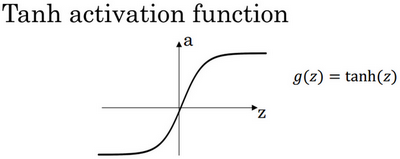
• tanh函数或者双曲正切函数（多数情况下优于sigmoid）：
  $$a=tanh(z)=\left[\begin{array}{c}\frac{e^z-e^{-z}}{e^z+e^{-z}}\end{array}\right]$$
  $$g^{\prime }(z)=1-a^2$$
  
• ReLu 函数 rectified linear unit：（most）
  $$a=g(z)=max(0,z)$$
  $$g^{\prime }(z)=\{\begin{array}{ll}0& \text{if z<0}\\ 1& \text{if z>0}\\ undefined& \text{if z=0}\end{array}$$
  (在z=0时没有定义，但是在实际应用中可以赋值成1或0即改第二项为 if z>=0，当然z=0的情况很少)
• Leaky ReLu
  $$a=g(z)=max(0.01z,z)$$
  $$g^{\prime }(z)=\{\begin{array}{ll}0.01& \text{if z<0}\\ 1& \text{if z>0}\\ undefined& \text{if z=0}\end{array}$$
• 线性激活函数:隐藏单元不能使用，机器学习中的回归问题输出层可能可以使用
  $$g(z)=z$$

神经网络的梯度下降

layers:

• n^[0] = n_x
• n^[1] = 层数（4)
• n^[2] = 1

parameters：

• w^[1] (n^[1]，n^[0])
• b^[1] (n^[1]，1)
• w^[2] (n^[2]，n^[1])
• b^[2] (n^[2]，1)
  
  dz^[1]= W^[2]Tdz^[2] * g^[1]’(z^[1])

随机初始化

使所有隐藏单元计算相同的函数由于对称原则
w 随机且取较小值，如果较大使得z较大，则在ReLu函数中处于斜率较为平缓的位置，会导致梯度下降迭代速度变慢。b可以初始化为0。

W = np.random.rand((2,2))* 0.01
b = np.zero((2,1))

weekly test

a^[2](12) denotes the activation vector of the 2^nd layer for the 12^th training example.

a^[2]₄ is the activation output by the 4^thneuron of the 2^nd layer

#安装包的timeout问题

pip3 install --index-url https://pypi.douban.com/simple scipy

用pip(pip3)安装依赖包时默认访问https://pypi.python.org/simple/，但是经常出现不稳定以及访问速度非常慢的情况导致安装超时，此时可以换国内厂商提供的pipy镜像。

#查看pip安装属性

import pip._internal
print(pip._internal.pep425tags.get_supported())

Week 4 Deep Neural Network

核对矩阵的维度

z^[1] = w^[1] (np.dot) x + b
z^[l] = (n^[l], 1)
x(a^[0]) = (n^[0], 1)
w^[l] = (n^[l], n^[l-1])
vectorized
Z^[1] = (n^[1], m)
W^[1] = (n^[1], n^[0])
X = (n^[0], m)
b^[1] = (n^[1], 1)(remain the same, since the broadcasting of py)

z = wx + b

Remember that when we compute $WX+b$ in python, it carries out broadcasting. For example, if:

$$W=\left[\begin{array}{ccc}j& k& l\\ m& n& o\\ p& q& r\end{array}\right]X=\left[\begin{array}{ccc}a& b& c\\ d& e& f\\ g& h& i\end{array}\right]b=\left[\begin{array}{c}s\\ t\\ u\end{array}\right]$$

Then $WX+b$ will be:

$$WX+b=\left[\begin{array}{ccc}(ja+kd+lg)+s& (jb+ke+lh)+s& (jc+kf+li)+s\\ (ma+nd+og)+t& (mb+ne+oh)+t& (mc+nf+oi)+t\\ (pa+qd+rg)+u& (pb+qe+rh)+u& (pc+qf+ri)+u\end{array}\right]$$