


一 实例描述
构建网络模型完成将3类样本分开的任务。
在实现过程中先生成3类样本模拟数据,构造神经网络,通过softmax分类的方法计算神经网络的输出值,并将其分开。
二 代码
import tensorflow as tf
import numpy as np
import matplotlib.pyplot as plt
from sklearn.utils import shuffle
from matplotlib.colors import colorConverter, ListedColormap
'''
使用generate函数,生成2000个点,3类数据,并且使用one_hot编码
'''
# 对于上面的fit可以这么扩展变成动态的
from sklearn.preprocessing import OneHotEncoder
def onehot(y,start,end):
ohe = OneHotEncoder()
a = np.linspace(start,end-1,end-start)
b =np.reshape(a,[-1,1]).astype(np.int32)
ohe.fit(b)
c=ohe.transform(y).toarray()
return c
#
def generate(sample_size, num_classes, diff,regression=False):
np.random.seed(10)
mean = np.random.randn(2)
cov = np.eye(2)
#len(diff)
samples_per_class = int(sample_size/num_classes)
X0 = np.random.multivariate_normal(mean, cov, samples_per_class)
Y0 = np.zeros(samples_per_class)
for ci, d in enumerate(diff):
X1 = np.random.multivariate_normal(mean+d, cov, samples_per_class)
Y1 = (ci+1)*np.ones(samples_per_class)
X0 = np.concatenate((X0,X1))
Y0 = np.concatenate((Y0,Y1))
#print(X0, Y0)
if regression==False: #one-hot 0 into the vector "1 0
Y0 = np.reshape(Y0,[-1,1])
#print(Y0.astype(np.int32))
Y0 = onehot(Y0.astype(np.int32),0,num_classes)
#print(Y0)
X, Y = shuffle(X0, Y0)
#print(X, Y)
return X,Y
# Ensure we always get the same amount of randomness
np.random.seed(10)
input_dim = 2
num_classes =3
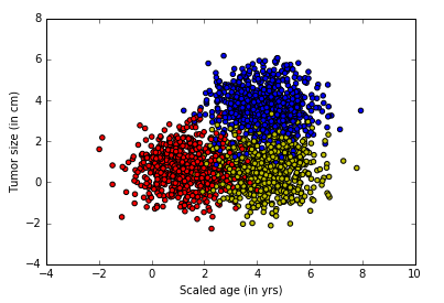
X, Y = generate(2000,num_classes, [[3.0],[3.0,0]],False)
aa = [np.argmax(l) for l in Y]
colors =['r' if l == 0 else 'b' if l==1 else 'y' for l in aa[:]]
plt.scatter(X[:,0], X[:,1], c=colors)
plt.xlabel("Scaled age (in yrs)")
plt.ylabel("Tumor size (in cm)")
plt.show()
'''
构建网络模型
使用softmax分类,损失函数loss仍然使用交叉熵,对于错误率评估换成了one_hot结果里面不相同的个数,优化器使用AdamOptimizer
'''
lab_dim = num_classes
# tf Graph Input
input_features = tf.placeholder(tf.float32, [None, input_dim])
input_lables = tf.placeholder(tf.float32, [None, lab_dim])
# Set model weights
W = tf.Variable(tf.random_normal([input_dim,lab_dim]), name="weight")
b = tf.Variable(tf.zeros([lab_dim]), name="bias")
output = tf.matmul(input_features, W) + b
z = tf.nn.softmax( output )
a1 = tf.argmax(tf.nn.softmax( output ), axis=1)#按行找出最大索引,生成数组
b1 = tf.argmax(input_lables, axis=1)
err = tf.count_nonzero(a1-b1) #两个数组相减,不为0的就是错误个数
cross_entropy = tf.nn.softmax_cross_entropy_with_logits( labels=input_lables,logits=output)
loss = tf.reduce_mean(cross_entropy)#对交叉熵取均值很有必要
optimizer = tf.train.AdamOptimizer(0.04) #尽量用这个--收敛快,会动态调节梯度
train = optimizer.minimize(loss) # let the optimizer train
'''
设置参数进行训练
设置数据集迭代50次,每次的minibatchSize取25条。
'''
maxEpochs = 50
minibatchSize = 25
# 启动session
with tf.Session() as sess:
sess.run(tf.global_variables_initializer())
for epoch in range(maxEpochs):
sumerr=0
for i in range(np.int32(len(Y)/minibatchSize)):
x1 = X[i*minibatchSize:(i+1)*minibatchSize,:]
y1 = Y[i*minibatchSize:(i+1)*minibatchSize,:]
_,lossval, outputval,errval = sess.run([train,loss,output,err], feed_dict={input_features: x1, input_lables:y1})
#错误率的计算,每一次计算都会将err错误值累加,数据集迭代完一次完成err的错误率进行一次平均,然后在输出平均值
sumerr =sumerr+(errval/minibatchSize)
print ("Epoch:", '%04d' % (epoch+1), "cost=","{:.9f}".format(lossval),"err=",sumerr/(np.int32(len(Y)/minibatchSize)))
'''
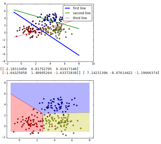
三分类问题,线性可分是怎样分的?先取200个测试的点,在图像中显示出来,接着将模型中x1和x2的映射关系以一条直线的方式显示出来。因为输出有3类,所以相当于有3条直线
'''
train_X, train_Y = generate(200,num_classes, [[3.0],[3.0,0]],False)
aa = [np.argmax(l) for l in train_Y]
colors =['r' if l == 0 else 'b' if l==1 else 'y' for l in aa[:]]
plt.scatter(train_X[:,0], train_X[:,1], c=colors)
x = np.linspace(-1,8,200)
y=-x*(sess.run(W)[0][0]/sess.run(W)[1][0])-sess.run(b)[0]/sess.run(W)[1][0]
plt.plot(x,y, label='first line',lw=3)
y=-x*(sess.run(W)[0][1]/sess.run(W)[1][1])-sess.run(b)[1]/sess.run(W)[1][1]
plt.plot(x,y, label='second line',lw=2)
y=-x*(sess.run(W)[0][2]/sess.run(W)[1][2])-sess.run(b)[2]/sess.run(W)[1][2]
plt.plot(x,y, label='third line',lw=1)
plt.legend()
plt.show()
'''
3个权重分别代表3条直线,还原成模型就是模型里的3个输出的分类节点
第一个输出节点代表分类0,红色,蓝线。
第二个输出节点代表分类1,蓝色,绿线
第三个输出节点代表分类2,红色,红线
这3条直接的斜率和截距是由神经网络的学习参数转化而来的。在神经网络里,一个样本通过这3个公式会得到3个结果,这3个结果可以理解成3个类的特征值。其中哪个值最大,则表示该样本具有哪种
类别的特征值最强烈,即属于哪一类。这3条线也没有把集合点分开,这是因为它们分类规则不一样的。
回顾一下直线公式:y=-x*(w1/w2)-(b/w2)
正常来讲:如果一个点在直线上,等式成立;如果点在直线上方,那么左边的y值就大,如果点在直线下方,那么右边的算式值就大。
当放到模型中对应的图像并不是这样的,还取决于w1的正负取值,当w1为负值,情况是相反的。从输出来看,只有第一条线(蓝色)的w1是负,所以蓝线是取下面的点,红线和绿线是取下方的点。
'''
print(sess.run(W),sess.run(b))
'''
模型可视化
'''
train_X, train_Y = generate(200,num_classes, [[3.0],[3.0,0]],False)
aa = [np.argmax(l) for l in train_Y]
colors =['r' if l == 0 else 'b' if l==1 else 'y' for l in aa[:]]
plt.scatter(train_X[:,0], train_X[:,1], c=colors)
nb_of_xs = 200
xs1 = np.linspace(-1, 8, num=nb_of_xs)
xs2 = np.linspace(-1, 8, num=nb_of_xs)
xx, yy = np.meshgrid(xs1, xs2) # 创建登高线
# Initialize and fill the classification plane
classification_plane = np.zeros((nb_of_xs, nb_of_xs))
for i in range(nb_of_xs):
for j in range(nb_of_xs):
#classification_plane[i,j] = nn_predict(xx[i,j], yy[i,j])
classification_plane[i,j] = sess.run(a1, feed_dict={input_features: [[ xx[i,j], yy[i,j] ]]} )
# Create a color map to show the classification colors of each grid point
cmap = ListedColormap([
colorConverter.to_rgba('r', alpha=0.30),
colorConverter.to_rgba('b', alpha=0.30),
colorConverter.to_rgba('y', alpha=0.30)])
# Plot the classification plane with decision boundary and input samples
plt.contourf(xx, yy, classification_plane, cmap=cmap)
plt.show()
三 运行结果
...
Epoch: 0042 cost= 0.421706438 err= 0.0881012658228
Epoch: 0043 cost= 0.422015101 err= 0.0881012658228
Epoch: 0044 cost= 0.422297388 err= 0.0881012658228
Epoch: 0045 cost= 0.422555774 err= 0.0881012658228
Epoch: 0046 cost= 0.422792047 err= 0.0881012658228
Epoch: 0047 cost= 0.423008054 err= 0.0881012658228
Epoch: 0048 cost= 0.423205525 err= 0.0881012658228
Epoch: 0049 cost= 0.423386186 err= 0.0881012658228
Epoch: 0050 cost= 0.423551381 err= 0.0881012658228
四 说明
将三分类模型用不同的颜色区域进行区分,这样就符合人眼规律一个比较直观的可视化图样了。


 4万+
4万+

 被折叠的 条评论
为什么被折叠?
被折叠的 条评论
为什么被折叠?
 到【灌水乐园】发言


