线性回归（python实战）

线性回归（python实战）

线性回归目标函数

线性回归（理论篇）中推导了线性回归的目标函数为：

$$J(\theta) = \sum^N(\theta x - y )^2$$

梯度下降法求解参数

梯度下降法迭代公式为：

$$\theta := \theta - \alpha \sum^N(\sum^m (x_{i}\theta_{i} - y_{i})x_{i})$$
其中 $\alpha$为学习率。

python3 实战

import numpy as np
import matplotlib.pyplot as plt

随机梯度下降

• @param X numpy.array m*n
• @param Y numpy.array m*1
• @param alpha 学习率
• @param theta 参数初始值 numpy.array n
• @param max_iter 最大迭代次数
• @param eps 精度

def stochasticGradientDescent(X,Y,alpha = 0.01,theta = None,max_iter = 1000,eps = 1e-5):
    if theta is None:
        theta = np.zeros([X.shape[1]])
    for iter in range(max_iter):
        for index,x in enumerate(X):
            # 梯度
            gradient = (np.dot(x,theta) - Y[index]) * x 
            # 对梯度做归一化,防止梯度过大导致变化剧烈
            diff = gradient / np.power(np.dot(gradient,gradient),0.5) * alpha
            theta = theta - diff
             # 如果增量小于精度，则迭代结束
            if np.max(np.fabs(diff)) < eps :
                return theta
    return theta

批量梯度下降

• @param X numpy.array m*n
• @param Y numpy.array m*1
• @param alpha 学习率
• @param theta 参数初始值 numpy.array n
• @param max_iter 最大迭代次数
• @param eps 精度

def gradientDescent(X,Y,alpha = 0.01,theta = None,max_iter = 1000,eps = 1e-5):
    N = X.shape[0]
    if theta is None:
        theta = np.zeros([X.shape[1]])
    for iter in range(max_iter):
        gradient = np.dot((np.dot(X,theta) - Y.flatten()) ,X )
        diff = alpha *  gradient / np.power(np.dot(gradient,gradient),0.5)
        theta = theta - diff
        if np.max(np.fabs(diff)) < eps :
            return theta
    return theta

小批量梯度下降

• @param X numpy.array m*n
• @param Y numpy.array m*1
• @min_batch 最小样本数
• @param alpha 学习率
• @param theta 参数初始值 numpy.array n
• @param max_iter 最大迭代次数
• @param eps 精度

def batchGradientDescent(X,Y,min_batch = 1,alpha = 0.01,theta = None,max_iter = 1000,eps = 1e-5):
    if theta is None:
        theta = np.zeros([X.shape[1]])
    for iter in range(max_iter):
        # 如果样本数不是最小样本数的整倍数，补齐
        remainder = X.shape[0] % min_batch
        X_tmp = X
        Y_tmp = Y
        if(remainder != 0):
            X_tmp = np.concatenate((X_tmp,X[0 : (min_batch - remainder),:]))
            Y_tmp = np.concatenate((Y_tmp,Y[0 : (min_batch - remainder),:]))
        for batch in range(0, X.shape[0] , min_batch): 
            X_batch = X_tmp[batch : batch + min_batch,:]
            Y_batch = Y_tmp[batch : batch + min_batch,:]
            gradient = np.dot((np.dot(X_batch,theta) - Y_batch.flatten()) ,X_batch )
            diff = alpha *  gradient / np.power(np.dot(gradient,gradient),0.5) 
            theta = theta - diff
            if np.max(np.fabs(diff)) < eps :
                return theta
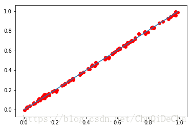
    return theta

线性回归拟合直线 y = x

# 随机生成0-1之间的100个数，计算y=x并加上均值为0方差为0.1的高斯噪声
size = [100,1]
x_train = np.random.RandomState(0).random_sample(size) 
y_train = x_train + np.random.normal(0, 0.01, size)

# x的增广矩阵
x_train = np.c_[np.ones(size),x_train]

# 小批量梯度下降求解参数
theta = batchGradientDescent(x_train,y_train,10)

theta

array([2.03633491e-04, 1.01366885e+00])

x_test = np.arange(100)/100
y_test = theta[0] + theta[1] * x_test
plt.scatter(x_train[:,1],y_train,color="red")
plt.plot(x_test,y_test)

[<matplotlib.lines.Line2D at 0x7f2d658e9c18>]

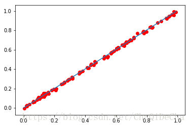
# 随机梯度下降
theta = stochasticGradientDescent(x_train,y_train)

theta

array([-0.00326086,  1.00808704])

x_test = np.arange(100)/100
y_test = theta[0] + theta[1] * x_test
plt.scatter(x_train[:,1],y_train,color="red")
plt.plot(x_test,y_test)

[<matplotlib.lines.Line2D at 0x7f2d62b000b8>]

# 批量梯度下降
theta = gradientDescent(x_train,y_train)

theta

array([-7.81797726e-04,  1.00543598e+00])

x_test = np.arange(100)/100
y_test = theta[0] + theta[1] * x_test
plt.scatter(x_train[:,1],y_train,color="red")
plt.plot(x_test,y_test)

[<matplotlib.lines.Line2D at 0x7f2d62a73b00>]

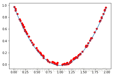
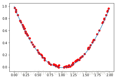
高阶拟合

线性回归是指参数是线性的，可以用来拟合高阶曲线

# 随机生成0-2之间的100个数，计算y=x^2 - 2x + 1并加上均值为0方差为0.1的高斯噪声
size = [100,1]
x = np.random.RandomState(0).random_sample(size) * 2
y_train = np.power(x ,2) - 2 * x  + 1 + np.random.normal(0, 0.01, size)

x_train = np.c_[np.ones(size),x,np.power(x,2)]

theta = stochasticGradientDescent(x_train,y_train)

theta

array([ 0.98408282, -1.99729037,  0.99756586])

plt.scatter(x_train[:,1],y_train,color = 'red')
x_test = np.arange(200) / 100
y_test = theta[2] * np.power(x_test ,2) + theta[1] * x_test  + theta[0]
plt.plot(x_test,y_test)

[<matplotlib.lines.Line2D at 0x7f2d6282b4e0>]

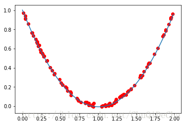
theta = gradientDescent(x_train,y_train)

theta

array([ 1.00163361, -2.0060185 ,  0.99703326])

plt.scatter(x_train[:,1],y_train,color = 'red')
x_test = np.arange(200) / 100
y_test = theta[2] * np.power(x_test ,2) + theta[1] * x_test  + theta[0]
plt.plot(x_test,y_test)

[<matplotlib.lines.Line2D at 0x7f2d627c08d0>]

theta = batchGradientDescent(x_train,y_train,10)

theta

array([ 0.99796869, -1.99954664,  0.99281468])

plt.scatter(x_train[:,1],y_train,color = 'red')
x_test = np.arange(200) / 100
y_test = theta[2] * np.power(x_test ,2) + theta[1] * x_test  + theta[0]
plt.plot(x_test,y_test)

[<matplotlib.lines.Line2D at 0x7f2d6277aac8>]