PS:
1,本文博文的matlab代码分析自:SIFT算法的“始作俑者”-----lowe,
2,网址为:http://www.cs.ubc.ca/~lowe/keypoints/
3,下面的代码均来自于他的SIFT算法(改写了一部分代码),此算法有其专利,专利拥有者为英属哥伦比亚大学。
4,本文只是感性的认知和使用SIFT算法,对深入的数学原理未做详尽探讨。
1,SIFT算法的实质是在不同的尺度空间上查找关键点(特征点),并计算出关键点的方向。SIFT所查找到的关键点是一些十分突出,不会因光照,仿射变换和噪音等因素而变化的点,如角点、边缘点、暗区的亮点及亮区的暗点等。
a,不变性:
——对图像的旋转和尺度变化具有不变性;
——对三维视角变化和光照变化具有很强的适应性;
——局部特征,在遮挡和场景杂乱时仍保持不变性;
b,辨别力强:
——特征之间相互区分的能力强,有利于匹配;
c,数量较多:
——Lowe原话:一般500*500的图像能提取约2000个特征点(这个数字依赖于图像内容和几个参数的选择)。
在高斯差分(Difference of Gaussian,DOG)尺度空间中提取极值点并进行优化,从而获取特征点。

2,SIFT算法点检测的具体步骤:
——构建尺度空间;
——构造高斯差分尺度空间;
——DoG尺度空间极值点检测;
——特征点精确定位;
——去除不稳定点;
3,OpenCV下SIFT特征点提取与匹配的大致流程如下:
读取图片-》特征点检测(位置,角度,层)-》特征点描述的提取(16*8维的特征向量)-》匹配-》显示
其中,特征点提取主要有两个步骤,下面做具体分析。
1、使用opencv内置的库读取两幅图片
2、生成一个SiftFeatureDetector的对象,这个对象顾名思义就是SIFT特征的探测器,用它来探测一副图片中SIFT点的特征,存到一个KeyPoint类型的vector中。这里有必要说keypoint的数据结构,涉及内容较多,具体分析查看opencv中keypoint数据结构分析,里面讲的自认为讲的还算详细(表打我……)。简而言之最重要的一点在于:
keypoint只是保存了opencv的sift库检测到的特征点的一些基本信息,但sift所提取出来的特征向量其实不是在这个里面,特征向量通过SiftDescriptorExtractor 提取,结果放在一个Mat的数据结构中。这个数据结构才真正保存了该特征点所对应的特征向量。具体见后文对SiftDescriptorExtractor 所生成的对象的详解。
就因为这点没有理解明白耽误了一上午的时间。哭死!
3、对图像所有KEYPOINT提取其特征向量:
得到keypoint只是达到了关键点的位置,方向等信息,并无该特征点的特征向量,要想提取得到特征向量就还要进行SiftDescriptorExtractor 的工作,建立了SiftDescriptorExtractor 对象后,通过该对象,对之前SIFT产生的特征点进行遍历,找到该特征点所对应的128维特征向量。具体方法参见opencv中SiftDescriptorExtractor所做的SIFT特征向量提取工作简单分析。通过这一步后,所有keypoint关键点的特征向量被保存到了一个MAT的数据结构中,作为特征。
4、对两幅图的特征向量进行匹配,得到匹配值。
两幅图片的特征向量被提取出来后,我们就可以使用BruteForceMatcher对象对两幅图片的descriptor进行匹配,得到匹配的结果到matches中,这其中具体的匹配方法暂没细看,过段时间补上。
至此,SIFT从特征点的探测到最后的匹配都已经完成,虽然匹配部分不甚了解,只扫对于如何使用OPENCV进行sift特征的提取有了一定的理解。接下来可以开始进行下一步的工作了。
一,源代码中三个主要函数
1,共有三段Matlab代码源文件
1)match.m:测试程序
功能:该函数读入两幅(灰度)图像,找出各自的 SIFT 特征, 并显示两连接两幅图像中被匹配的特征点(关键特征点(the matched keypoints)直线(将对应特征点进行连接)。判断匹配的准则是匹配距离小于distRatio倍于下一个最近匹配的距离( A match is accepted only if its distance is less than distRatio times the distance to the second closest match.
该程序返回显示的匹配对的数量。( It returns the number of matches displayed.)
调用实例: match('desk.jpg','book.jpg');
( 假如,想测试一个含有一本书的桌面的图像 和一本书的图像之间特征匹配)
调用方法和参数描述:略。
注意:
(a)图像为灰度图像,如果是彩色图像,应该在调用前利用rgb2gray转换为灰度图像。
(b)参数distRatio 为控制匹配点数量的系数,这里取 0.6,该参数决定了匹配点的数量,在Match.m文件中调整该参数,获得最合适的匹配点数量。
2)sift.m :尺度不变特征变换(SIFT算法)的核心算法程序
具体原理详见David G. Lowe发表于2004年Int Journal of Computer Vision,2(60):91-110的那篇标题为“Distivtive Image Features from Scale -Invariant Keypoints" 的论文
功能:该函数读入灰度图像,返回SIFT 特征关键点( SIFT keypoints.)
调用方法和参数描述:
调用方式:[image, descriptors, locs] = sift(imageFile)
输入参数( Input parameters): imageFile: 图像文件名.
输出或返回参数( Returned): image: 是具有double format格式的图像矩阵
descriptors: 一个 K-by-128 的矩阵x, 其中每行是针对找到的K个关键特征点(the K keypoints)的不变量描述子. 这个描述子(descriptor)是一个拥有128个数值并归一化为单位长度向量.
locs: 是K-by-4 矩阵, 其中的每一行具有四个数值,表示关键点位置信息 (在图像中的行坐标,列坐标(row, column) ,注意,一般图像的左上角为坐标原点), 尺度scale,高斯尺度空间的参数,其中该参数也决定了frame(结构)确定的图像disk的大小, 最后一个参数是方向orientation). 方向参数的范围是[-PI, PI] 单位为弧度.
3)appendimages.m: 该函数创建一个新的图像分别包含两个匹配的图像和他们之间的匹配对的连接直线.
二,小应用
SIFT算法解决图像平移的小应用:
- close all;
- clear all;
- clc;
-
- %读取自用图片,(如果是彩色图像将会被sift函数自动转换成灰度图处理)
- i1=imread('image2_1.jpg');
- i2=imread('a2.jpg');
- imwrite(i1,'v1.jpg','quality',80);
- imwrite(i2,'v2.jpg','quality',80);
-
- %找到每一幅图的“SIFT关键点”
- [im1, des1, loc1] = sift('v1.jpg');
- [im2, des2, loc2] = sift('v2.jpg');
-
- %显示关键点及其方向矢量信息
- showkeys(im1, loc1);
- showkeys(im2, loc2);
-
-
- % For efficiency in Matlab, it is cheaper to compute dot products between
- % unit vectors rather than Euclidean distances. Note that the ratio of
- % angles (acos of dot products of unit vectors) is a close approximation
- % to the ratio of Euclidean distances for small angles.
- %
- % distRatio: Only keep matches in which the ratio of vector angles from the
- % nearest to second nearest neighbor is less than distRatio.
-
- distRatio = 0.6;%控制匹配点数量的系数,这里取 0.6,该参数决定了匹配点的数量。
-
- % For each descriptor in the first image, select its match to second image.
- des2t = des2'; % Precompute matrix transpose
- len=size(des1,1);
- for i = 1 : len
- dotprods = des1(i,:) * des2t; % Computes vector of dot products
- [vals,indx] = sort(acos(dotprods)); % Take inverse cosine and sort results
-
- % Check if nearest neighbor has angle less than distRatio times 2nd.
- % 检查是否最近邻域有角度小于二倍distratio。
- if (vals(1) < distRatio * vals(2))
- match(i) = indx(1);
- else
- match(i) = 0;
- end
- end
-
- %将两幅图像显示在一起
- im3 = appendimages(im1,im2);
-
- %将匹配点连在一起
- figure('Position', [100 100 size(im3,2) size(im3,1)]);
- colormap('gray');
- imagesc(im3);
- hold on;
- cols1 = size(im1,2);
- %loc (row, column, scale, orientation)
- tran_col = 0;
- tran_row = 0;
- for i = 1: size(des1,1)
- if (match(i) > 0)
- col1=loc1(i,2);
- row1=loc1(i,1);
- col2=loc2(match(i),2);
- row2=loc2(match(i),1);
- tran_col=tran_col+col2-col1;
- tran_row=tran_row+row2-row1;
- line([loc1(i,2), loc2(match(i),2)+cols1],[loc1(i,1), loc2(match(i),1)], 'Color', 'c');%将两个匹配点连接
- end
- end
- hold off;
- %打印匹配点个数
- num = sum(match > 0);
- tran_col = int32(tran_col/num);
- tran_row = int32(tran_row/num);
- fprintf('Found %d matches.\n', num);
- fprintf('列偏移量%d.\n', tran_col);
- fprintf('行偏移量%d.\n', tran_row);
-
- vv2=imread('v2.jpg');
- %平移回去
- figure,imshow(i1);
- se=translate(strel(1),[double(-tran_row),double(-tran_col)] );
- img2=imdilate(vv2,se);
- figure,imshow(img2);
OpenCV写得图像配准(SIFT算法)
- #include<iostream>
- #include <opencv2/highgui/highgui.hpp>
- #include "opencv2/core/core.hpp"
- #include "highgui.h"
- #include "opencv2/imgproc/imgproc.hpp"
- #include "opencv2/features2d/features2d.hpp"
- #include "opencv2/nonfree/nonfree.hpp"
- #include "opencv2/legacy/legacy.hpp"
-
- using namespace cv;
- using namespace std;
-
- int main(int argc, char** argv)
- {
-
- Mat img1 = imread("a1.jpg");
- Mat img2 = imread("a2.jpg");
-
- SIFT sift1, sift2;
-
- vector<KeyPoint> key_points1, key_points2;
-
- Mat descriptors1, descriptors2, mascara;
-
- sift1(img1, mascara, key_points1, descriptors1);
- sift2(img2, mascara, key_points2, descriptors2);
-
-
- BruteForceMatcher<L2<float>> matcher;
-
- vector<DMatch>matches;
-
- matcher.match(descriptors1, descriptors2, matches);
-
-
- std::nth_element(matches.begin(),
- matches.begin() + 29,
- matches.end());
-
- matches.erase(matches.begin() + 30, matches.end());
-
- namedWindow("SIFT_matches");
- Mat img_matches;
-
- drawMatches(img1, key_points1,
- img2, key_points2,
- matches,
- img_matches,
- Scalar(255, 0, 255));
- imshow("SIFT_matches", img_matches);
- waitKey(0);
- return 0;
- }
配准效果(图像存在刚性平移):
OpenCV中的SURF算法解决平移问题:
- #include <opencv2/legacy/legacy.hpp>
- #include <opencv2/nonfree/nonfree.hpp>//opencv_nonfree模块:包含一些拥有专利的算法,如SIFT、SURF函数源码。
- #include <stdio.h>
- #include <iostream>
- #include "opencv2/core/core.hpp"
- #include "opencv2/features2d/features2d.hpp"
- #include "opencv2/highgui/highgui.hpp"
- #include <opencv2/nonfree/features2d.hpp>
- #include "vector"
- using namespace cv;
- using namespace std;
-
-
- void translateTransform(cv::Mat const& src, cv::Mat& dst, int dx, int dy)
- {
-
- const int rows = src.rows;
- const int cols = src.cols;
-
- dst.create(rows, cols, src.type());
-
- for (int i = 0; i < rows; i++)
- {
- for (int j = 0; j < cols; j++)
- {
-
- int x = j - dx;
- int y = i - dy;
-
- if (x >= 0 && y >= 0 && x < cols && y < rows)
- dst.at<uchar>(i, j) = src.at<uchar>(y, x);
- else
- dst.at<uchar>(i, j) = src.at<uchar>(i, j);
- }
- }
- }
-
-
- int main(int argc, char** argv)
- {
- Mat img_11 = imread("a1.jpg");
- Mat img_22 = imread("a2.jpg");
-
- if (!img_11.data || !img_22.data)
- {
- std::cout << " --(!) Error reading images " << std::endl;
- return -1;
- }
- Mat img_1, img_2;
- cvtColor(img_11, img_1, CV_BGR2GRAY);
- cvtColor(img_22, img_2, CV_BGR2GRAY);
-
- int minHessian = 40;
-
-
- SurfFeatureDetector detector( minHessian );
-
- std::vector<KeyPoint> keypoints_1, keypoints_2;
-
- detector.detect(img_1, keypoints_1);
- detector.detect(img_2, keypoints_2);
-
-
-
- SurfDescriptorExtractor extractor;
-
- Mat descriptors_1, descriptors_2;
-
- extractor.compute(img_1, keypoints_1, descriptors_1);
- extractor.compute(img_2, keypoints_2, descriptors_2);
-
-
- FlannBasedMatcher matcher;
- std::vector< DMatch > matches;
- matcher.match(descriptors_1, descriptors_2, matches);
-
- double max_dist = 0; double min_dist = 100;
-
-
- for (int i = 0; i < descriptors_1.rows; i++)
- {
- double dist = matches[i].distance;
- if (dist < min_dist) min_dist = dist;
- if (dist > max_dist) max_dist = dist;
- }
-
- printf("-- Max dist : %f \n", max_dist);
- printf("-- Min dist : %f \n", min_dist);
-
-
-
- std::vector< DMatch > good_matches;
-
- for (int i = 0; i < descriptors_1.rows; i++)
- {
- if (matches[i].distance < 2 * min_dist)
- {
- good_matches.push_back(matches[i]);
- }
- }
-
-
- Mat img_matches;
- drawMatches(img_1, keypoints_1, img_2, keypoints_2,
- good_matches, img_matches, Scalar::all(-1), Scalar::all(-1),
- vector<char>(), DrawMatchesFlags::NOT_DRAW_SINGLE_POINTS);
-
-
- imshow("Good Matches", img_matches);
-
-
- int cnt_nums = 0;
- float tran_row = 0;
- float tran_col = 0;
- for ( unsigned int i = 0; i < good_matches.size(); i++)
- {
-
-
- float x1_zuo = keypoints_1[good_matches[i].queryIdx].pt.x;
- float y1_zuo = keypoints_1[good_matches[i].queryIdx].pt.y;
- float x2_zuo = keypoints_2[good_matches[i].trainIdx].pt.x;
- float y2_zuo = keypoints_2[good_matches[i].trainIdx].pt.y;
- printf("-- Good Match良性匹配点第[%d]个, 来自图1的关键点(坐标为 %f,%f):点的编号为 %d \n --来自图2的关键点(坐标为 %f,%f): 点的编号为 %d \n", i,
- keypoints_1[good_matches[i].queryIdx].pt.x, keypoints_1[good_matches[i].queryIdx].pt.y, good_matches[i].queryIdx,
- keypoints_2[good_matches[i].trainIdx].pt.x, keypoints_2[good_matches[i].trainIdx].pt.y, good_matches[i].trainIdx);
- tran_row += keypoints_2[good_matches[i].trainIdx].pt.x - keypoints_1[good_matches[i].queryIdx].pt.x;
- tran_col += keypoints_2[good_matches[i].trainIdx].pt.y - keypoints_1[good_matches[i].queryIdx].pt.y;
- cnt_nums++;
- }
- int tr_row = ceil(tran_row / cnt_nums);
- int tr_col = ceil(tran_col / cnt_nums);
- cout << "偏移量为:" << tr_row << " " << tr_col;
-
- Mat dst;
-
- translateTransform(img_2,dst,-tr_row,-tr_col);
-
- imshow("校准结果", dst);
-
- waitKey(0);
- return 0;
- }
注意:最后的匹配结果保存在vector<DMatch>中。DMatch用来保存匹配后的结果
- struct DMatch
- {
- DMatch() :
- queryIdx(-1), trainIdx(-1), imgIdx(-1), distance(std::numeric_limits<float>::max()) {}
- DMatch(int _queryIdx, int _trainIdx, float _distance) :
- queryIdx(_queryIdx), trainIdx(_trainIdx), imgIdx(-1), distance(_distance) {}
- DMatch(int _queryIdx, int _trainIdx, int _imgIdx, float _distance) : queryIdx(_queryIdx), trainIdx(_trainIdx), imgIdx(_imgIdx), distance(_distance) {}
- int queryIdx;
- int trainIdx;
- int imgIdx;
- float distance;
- bool operator < (const DMatch &m) const;
- };
该校准结果是对上面这幅图中右边这幅偏移图像的校准结果,但是明显的问题是,边界问题没有处理好。
博文收录于转载:
一,图像配准算法小总结
首先,图像配准要素结合:特征空间,搜索空间,搜索策略,近似性度量;图像配准方法:
1.基于灰度信息的方法:交叉相关(互相关)方法,相关系数度量,序贯相似检测算法,信息理论的交换信息相似性准则。
2.基于变换域的方法:相位相关法,Walsh Transform变换。
3.基于特征的方法:常用的图像特征有:特征点(包括角点、高曲率点等)、直线段、边缘(Robert、高斯-拉普拉斯LoG、Canny、Gabor滤波等边缘检测算子)或轮廓、闭合区域、特征结构以及统计特征如矩不变量等。
注:像素灰度信息的互相关算法相比,特征提取包含了高层信号信息,所以该类算法对光照、噪声等的抗干扰能力强。
常用的空间变换模型:刚体变换(平移、旋转与缩放的组合)、仿射变换、透射变换、投影变换、非线性变换。
常用的相似性测度:
1.距离测度:均方根误差,差绝对值和误差,兰氏距离,Mahalanobis距离,绝对差,Hausdorff距离等。
2.角度度量法(概率测度)。
3.相关度量法
配准算法的评价标准:
配准时间、配准率、算法复杂度、算法的可移植性、算法的适用性、图像数据对算法的影响等(这里虽然不是目标追踪的评价标准,但是我们可以借鉴这些评价算法的标准)
二,图像配准算法分类
图像拼接技术主要包括两个关键环节即图像配准和图像融合对于图像融合部分,由于其耗时不太大,且现有的几种主要方法效果差别也不多,所以总体来说算法上比较成熟。而图像配准部分是整个图像拼接技术的核心部分,它直接关系到图像拼接算法的成功率和运行速度,因此配准算法的研究是多年来研究的重点。
目前的图像配准算法基本上可以分为两类:基于频域的方法(相位相关方法)和基于时域的方法。
相位相关法最早是由Kuglin和Hines在1975年提出的,并且证明在纯二维平移的情形下,拼接精度可以达到1个像素,多用于航空照片和卫星遥感图像的配准等领域。该方法对拼接的图像进行快速傅立叶变换,将两幅待配准图像变换到频域,然后通过它们的互功率谱直接计算出两幅图像间的平移矢量,从而实现图像的配准。由于其具有简单而精确的特点,后来成为最有前途的图像配准算法之一。但是相位相关方法一般需要比较大的重叠比例(通常要求配准图像之间有50%的重叠比例),如果重叠比例较小,则容易造成平移矢量的错误估计,从而较难实现图像的配准。
基于时域的方法又可具体分为基于特征的方法和基于区域的方法。基于特征的方法首先找出两幅图像中的特征点(如边界点、拐点),并确定图像间特征点的对应关系,然后利用这种对应关系找到两幅图像间的变换关系。这一类方法不直接利用图像的灰度信息,因而对光线变化不敏感,但对特征点对应关系的精确程度依赖很大。这一类方法采用的思想较为直观,目前大部分的图像配准算法都可以归为这一类。基于区域的方法是以一幅图像重叠区域中的一块作为模板,在另一幅图像中搜索与此模板最相似的匹配块,这种算法精度较高,但计算量过大。
按照匹配算法的具体实现又可以分为直接法和搜索法两大类,直接法主要包括变换优化法,它首先建立两幅待拼接图像间的变换模型,然后采用非线性迭代最小化算法直接计算出模型的变换参数,从而确定图像的配准位置。该算法效果较好,收敛速度较快,但是它要达到过程的收敛要求有较好的初始估计,如果初始估计不好,则会造成图像拼接的失败。搜索法主要是以一幅图像中的某些特征为依据,在另一幅图像中搜索最佳配准位置,常用的有比值匹配法,块匹配法和网格匹配法。比值匹配法是从一幅图像的重叠区域中部分相邻的两列上取出部分像素,然后以它们的比值作模板,在另一幅图像中搜索最佳匹配。这种算法计算量较小,但精度较低;块匹配法则是以一幅图像重叠区域中的一块作为模板,在另一幅图像中搜索与此模板最相似的匹配块,这种算法精度较高,但计算量过大;网格匹配法减小了块匹配法的计算量,它首先要进行粗匹配,每次水平或垂直移动一个步长,记录最佳匹配位置,然后在此位置附近进行精确匹配,每次步长减半,然后循环此过程直至步长减为0。这种算法较前两种运算量都有所减小,但在实际应用中仍然偏大,而且粗匹配时如果步长取的太大,很可能会造成较大的粗匹配误差,从而很难实现精确匹配。
参考资源:
【1】http://blog.csdn.net/zddblog/article/details/7521424
【2】http://www.cs.ubc.ca/~lowe/keypoints/
【3】http://blog.csdn.net/zhaocj/article/details/42124473
【4】http://www.cnblogs.com/cj695/p/4041478.html
【5】http://blog.csdn.net/llw01/article/details/9258699
【6】http://blog.csdn.net/xuluohongshang/article/details/52886352
注:本博文为EbowTang原创,后续可能继续更新本文。如果转载,请务必复制本条信息!
原文地址:http://blog.csdn.net/ebowtang/article/details/51236061
原作者博客:http://blog.csdn.net/ebowtang
PS:
1,本文博文的matlab代码分析自:SIFT算法的“始作俑者”-----lowe,
2,网址为:http://www.cs.ubc.ca/~lowe/keypoints/
3,下面的代码均来自于他的SIFT算法(改写了一部分代码),此算法有其专利,专利拥有者为英属哥伦比亚大学。
4,本文只是感性的认知和使用SIFT算法,对深入的数学原理未做详尽探讨。
1,SIFT算法的实质是在不同的尺度空间上查找关键点(特征点),并计算出关键点的方向。SIFT所查找到的关键点是一些十分突出,不会因光照,仿射变换和噪音等因素而变化的点,如角点、边缘点、暗区的亮点及亮区的暗点等。
a,不变性:
——对图像的旋转和尺度变化具有不变性;
——对三维视角变化和光照变化具有很强的适应性;
——局部特征,在遮挡和场景杂乱时仍保持不变性;
b,辨别力强:
——特征之间相互区分的能力强,有利于匹配;
c,数量较多:
——Lowe原话:一般500*500的图像能提取约2000个特征点(这个数字依赖于图像内容和几个参数的选择)。
在高斯差分(Difference of Gaussian,DOG)尺度空间中提取极值点并进行优化,从而获取特征点。
2,SIFT算法点检测的具体步骤:
——构建尺度空间;
——构造高斯差分尺度空间;
——DoG尺度空间极值点检测;
——特征点精确定位;
——去除不稳定点;
3,OpenCV下SIFT特征点提取与匹配的大致流程如下:
读取图片-》特征点检测(位置,角度,层)-》特征点描述的提取(16*8维的特征向量)-》匹配-》显示
其中,特征点提取主要有两个步骤,下面做具体分析。
1、使用opencv内置的库读取两幅图片
2、生成一个SiftFeatureDetector的对象,这个对象顾名思义就是SIFT特征的探测器,用它来探测一副图片中SIFT点的特征,存到一个KeyPoint类型的vector中。这里有必要说keypoint的数据结构,涉及内容较多,具体分析查看opencv中keypoint数据结构分析,里面讲的自认为讲的还算详细(表打我……)。简而言之最重要的一点在于:
keypoint只是保存了opencv的sift库检测到的特征点的一些基本信息,但sift所提取出来的特征向量其实不是在这个里面,特征向量通过SiftDescriptorExtractor 提取,结果放在一个Mat的数据结构中。这个数据结构才真正保存了该特征点所对应的特征向量。具体见后文对SiftDescriptorExtractor 所生成的对象的详解。
就因为这点没有理解明白耽误了一上午的时间。哭死!
3、对图像所有KEYPOINT提取其特征向量:
得到keypoint只是达到了关键点的位置,方向等信息,并无该特征点的特征向量,要想提取得到特征向量就还要进行SiftDescriptorExtractor 的工作,建立了SiftDescriptorExtractor 对象后,通过该对象,对之前SIFT产生的特征点进行遍历,找到该特征点所对应的128维特征向量。具体方法参见opencv中SiftDescriptorExtractor所做的SIFT特征向量提取工作简单分析。通过这一步后,所有keypoint关键点的特征向量被保存到了一个MAT的数据结构中,作为特征。
4、对两幅图的特征向量进行匹配,得到匹配值。
两幅图片的特征向量被提取出来后,我们就可以使用BruteForceMatcher对象对两幅图片的descriptor进行匹配,得到匹配的结果到matches中,这其中具体的匹配方法暂没细看,过段时间补上。
至此,SIFT从特征点的探测到最后的匹配都已经完成,虽然匹配部分不甚了解,只扫对于如何使用OPENCV进行sift特征的提取有了一定的理解。接下来可以开始进行下一步的工作了。
一,源代码中三个主要函数
1,共有三段Matlab代码源文件
1)match.m:测试程序
功能:该函数读入两幅(灰度)图像,找出各自的 SIFT 特征, 并显示两连接两幅图像中被匹配的特征点(关键特征点(the matched keypoints)直线(将对应特征点进行连接)。判断匹配的准则是匹配距离小于distRatio倍于下一个最近匹配的距离( A match is accepted only if its distance is less than distRatio times the distance to the second closest match.
该程序返回显示的匹配对的数量。( It returns the number of matches displayed.)
调用实例: match('desk.jpg','book.jpg');
( 假如,想测试一个含有一本书的桌面的图像 和一本书的图像之间特征匹配)
调用方法和参数描述:略。
注意:
(a)图像为灰度图像,如果是彩色图像,应该在调用前利用rgb2gray转换为灰度图像。
(b)参数distRatio 为控制匹配点数量的系数,这里取 0.6,该参数决定了匹配点的数量,在Match.m文件中调整该参数,获得最合适的匹配点数量。
2)sift.m :尺度不变特征变换(SIFT算法)的核心算法程序
具体原理详见David G. Lowe发表于2004年Int Journal of Computer Vision,2(60):91-110的那篇标题为“Distivtive Image Features from Scale -Invariant Keypoints" 的论文
功能:该函数读入灰度图像,返回SIFT 特征关键点( SIFT keypoints.)
调用方法和参数描述:
调用方式:[image, descriptors, locs] = sift(imageFile)
输入参数( Input parameters): imageFile: 图像文件名.
输出或返回参数( Returned): image: 是具有double format格式的图像矩阵
descriptors: 一个 K-by-128 的矩阵x, 其中每行是针对找到的K个关键特征点(the K keypoints)的不变量描述子. 这个描述子(descriptor)是一个拥有128个数值并归一化为单位长度向量.
locs: 是K-by-4 矩阵, 其中的每一行具有四个数值,表示关键点位置信息 (在图像中的行坐标,列坐标(row, column) ,注意,一般图像的左上角为坐标原点), 尺度scale,高斯尺度空间的参数,其中该参数也决定了frame(结构)确定的图像disk的大小, 最后一个参数是方向orientation). 方向参数的范围是[-PI, PI] 单位为弧度.
3)appendimages.m: 该函数创建一个新的图像分别包含两个匹配的图像和他们之间的匹配对的连接直线.
二,小应用
SIFT算法解决图像平移的小应用:
- close all;
- clear all;
- clc;
-
- %读取自用图片,(如果是彩色图像将会被sift函数自动转换成灰度图处理)
- i1=imread('image2_1.jpg');
- i2=imread('a2.jpg');
- imwrite(i1,'v1.jpg','quality',80);
- imwrite(i2,'v2.jpg','quality',80);
-
- %找到每一幅图的“SIFT关键点”
- [im1, des1, loc1] = sift('v1.jpg');
- [im2, des2, loc2] = sift('v2.jpg');
-
- %显示关键点及其方向矢量信息
- showkeys(im1, loc1);
- showkeys(im2, loc2);
-
-
- % For efficiency in Matlab, it is cheaper to compute dot products between
- % unit vectors rather than Euclidean distances. Note that the ratio of
- % angles (acos of dot products of unit vectors) is a close approximation
- % to the ratio of Euclidean distances for small angles.
- %
- % distRatio: Only keep matches in which the ratio of vector angles from the
- % nearest to second nearest neighbor is less than distRatio.
-
- distRatio = 0.6;%控制匹配点数量的系数,这里取 0.6,该参数决定了匹配点的数量。
-
- % For each descriptor in the first image, select its match to second image.
- des2t = des2'; % Precompute matrix transpose
- len=size(des1,1);
- for i = 1 : len
- dotprods = des1(i,:) * des2t; % Computes vector of dot products
- [vals,indx] = sort(acos(dotprods)); % Take inverse cosine and sort results
-
- % Check if nearest neighbor has angle less than distRatio times 2nd.
- % 检查是否最近邻域有角度小于二倍distratio。
- if (vals(1) < distRatio * vals(2))
- match(i) = indx(1);
- else
- match(i) = 0;
- end
- end
-
- %将两幅图像显示在一起
- im3 = appendimages(im1,im2);
-
- %将匹配点连在一起
- figure('Position', [100 100 size(im3,2) size(im3,1)]);
- colormap('gray');
- imagesc(im3);
- hold on;
- cols1 = size(im1,2);
- %loc (row, column, scale, orientation)
- tran_col = 0;
- tran_row = 0;
- for i = 1: size(des1,1)
- if (match(i) > 0)
- col1=loc1(i,2);
- row1=loc1(i,1);
- col2=loc2(match(i),2);
- row2=loc2(match(i),1);
- tran_col=tran_col+col2-col1;
- tran_row=tran_row+row2-row1;
- line([loc1(i,2), loc2(match(i),2)+cols1],[loc1(i,1), loc2(match(i),1)], 'Color', 'c');%将两个匹配点连接
- end
- end
- hold off;
- %打印匹配点个数
- num = sum(match > 0);
- tran_col = int32(tran_col/num);
- tran_row = int32(tran_row/num);
- fprintf('Found %d matches.\n', num);
- fprintf('列偏移量%d.\n', tran_col);
- fprintf('行偏移量%d.\n', tran_row);
-
- vv2=imread('v2.jpg');
- %平移回去
- figure,imshow(i1);
- se=translate(strel(1),[double(-tran_row),double(-tran_col)] );
- img2=imdilate(vv2,se);
- figure,imshow(img2);
OpenCV写得图像配准(SIFT算法)
- #include<iostream>
- #include <opencv2/highgui/highgui.hpp>
- #include "opencv2/core/core.hpp"
- #include "highgui.h"
- #include "opencv2/imgproc/imgproc.hpp"
- #include "opencv2/features2d/features2d.hpp"
- #include "opencv2/nonfree/nonfree.hpp"
- #include "opencv2/legacy/legacy.hpp"
-
- using namespace cv;
- using namespace std;
-
- int main(int argc, char** argv)
- {
-
- Mat img1 = imread("a1.jpg");
- Mat img2 = imread("a2.jpg");
-
- SIFT sift1, sift2;
-
- vector<KeyPoint> key_points1, key_points2;
-
- Mat descriptors1, descriptors2, mascara;
-
- sift1(img1, mascara, key_points1, descriptors1);
- sift2(img2, mascara, key_points2, descriptors2);
-
-
- BruteForceMatcher<L2<float>> matcher;
-
- vector<DMatch>matches;
-
- matcher.match(descriptors1, descriptors2, matches);
-
-
- std::nth_element(matches.begin(),
- matches.begin() + 29,
- matches.end());
-
- matches.erase(matches.begin() + 30, matches.end());
-
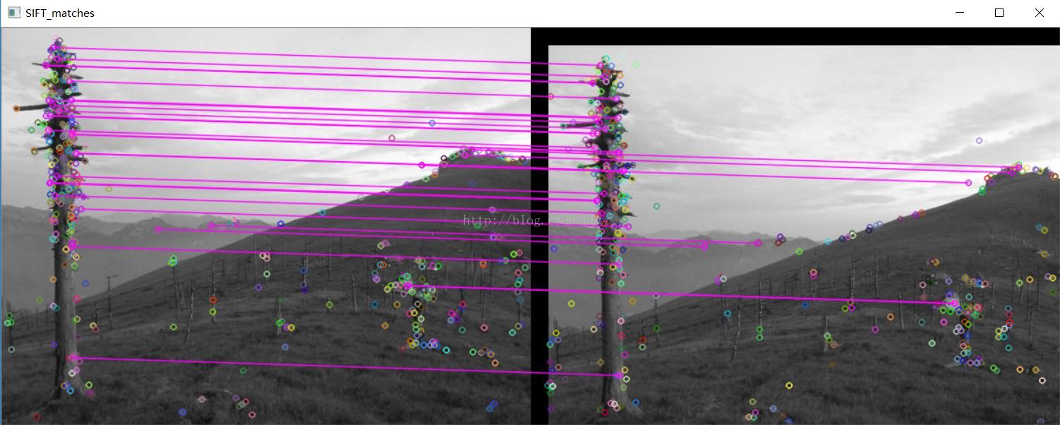
- namedWindow("SIFT_matches");
- Mat img_matches;
-
- drawMatches(img1, key_points1,
- img2, key_points2,
- matches,
- img_matches,
- Scalar(255, 0, 255));
- imshow("SIFT_matches", img_matches);
- waitKey(0);
- return 0;
- }
配准效果(图像存在刚性平移):
OpenCV中的SURF算法解决平移问题:
- #include <opencv2/legacy/legacy.hpp>
- #include <opencv2/nonfree/nonfree.hpp>//opencv_nonfree模块:包含一些拥有专利的算法,如SIFT、SURF函数源码。
- #include <stdio.h>
- #include <iostream>
- #include "opencv2/core/core.hpp"
- #include "opencv2/features2d/features2d.hpp"
- #include "opencv2/highgui/highgui.hpp"
- #include <opencv2/nonfree/features2d.hpp>
- #include "vector"
- using namespace cv;
- using namespace std;
-
-
- void translateTransform(cv::Mat const& src, cv::Mat& dst, int dx, int dy)
- {
-
- const int rows = src.rows;
- const int cols = src.cols;
-
- dst.create(rows, cols, src.type());
-
- for (int i = 0; i < rows; i++)
- {
- for (int j = 0; j < cols; j++)
- {
-
- int x = j - dx;
- int y = i - dy;
-
- if (x >= 0 && y >= 0 && x < cols && y < rows)
- dst.at<uchar>(i, j) = src.at<uchar>(y, x);
- else
- dst.at<uchar>(i, j) = src.at<uchar>(i, j);
- }
- }
- }
-
-
- int main(int argc, char** argv)
- {
- Mat img_11 = imread("a1.jpg");
- Mat img_22 = imread("a2.jpg");
-
- if (!img_11.data || !img_22.data)
- {
- std::cout << " --(!) Error reading images " << std::endl;
- return -1;
- }
- Mat img_1, img_2;
- cvtColor(img_11, img_1, CV_BGR2GRAY);
- cvtColor(img_22, img_2, CV_BGR2GRAY);
-
- int minHessian = 40;
-
-
- SurfFeatureDetector detector( minHessian );
-
- std::vector<KeyPoint> keypoints_1, keypoints_2;
-
- detector.detect(img_1, keypoints_1);
- detector.detect(img_2, keypoints_2);
-
-
-
- SurfDescriptorExtractor extractor;
-
- Mat descriptors_1, descriptors_2;
-
- extractor.compute(img_1, keypoints_1, descriptors_1);
- extractor.compute(img_2, keypoints_2, descriptors_2);
-
-
- FlannBasedMatcher matcher;
- std::vector< DMatch > matches;
- matcher.match(descriptors_1, descriptors_2, matches);
-
- double max_dist = 0; double min_dist = 100;
-
-
- for (int i = 0; i < descriptors_1.rows; i++)
- {
- double dist = matches[i].distance;
- if (dist < min_dist) min_dist = dist;
- if (dist > max_dist) max_dist = dist;
- }
-
- printf("-- Max dist : %f \n", max_dist);
- printf("-- Min dist : %f \n", min_dist);
-
-
-
- std::vector< DMatch > good_matches;
-
- for (int i = 0; i < descriptors_1.rows; i++)
- {
- if (matches[i].distance < 2 * min_dist)
- {
- good_matches.push_back(matches[i]);
- }
- }
-
-
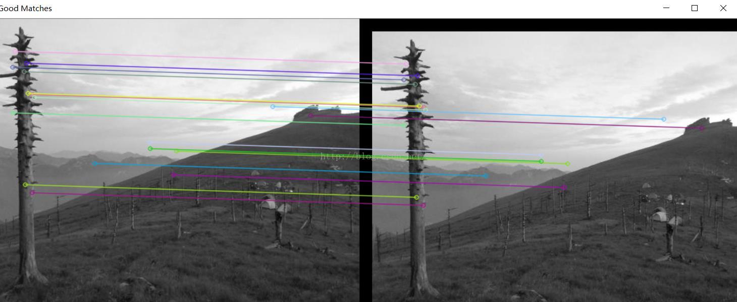
- Mat img_matches;
- drawMatches(img_1, keypoints_1, img_2, keypoints_2,
- good_matches, img_matches, Scalar::all(-1), Scalar::all(-1),
- vector<char>(), DrawMatchesFlags::NOT_DRAW_SINGLE_POINTS);
-
-
- imshow("Good Matches", img_matches);
-
-
- int cnt_nums = 0;
- float tran_row = 0;
- float tran_col = 0;
- for ( unsigned int i = 0; i < good_matches.size(); i++)
- {
-
-
- float x1_zuo = keypoints_1[good_matches[i].queryIdx].pt.x;
- float y1_zuo = keypoints_1[good_matches[i].queryIdx].pt.y;
- float x2_zuo = keypoints_2[good_matches[i].trainIdx].pt.x;
- float y2_zuo = keypoints_2[good_matches[i].trainIdx].pt.y;
- printf("-- Good Match良性匹配点第[%d]个, 来自图1的关键点(坐标为 %f,%f):点的编号为 %d \n --来自图2的关键点(坐标为 %f,%f): 点的编号为 %d \n", i,
- keypoints_1[good_matches[i].queryIdx].pt.x, keypoints_1[good_matches[i].queryIdx].pt.y, good_matches[i].queryIdx,
- keypoints_2[good_matches[i].trainIdx].pt.x, keypoints_2[good_matches[i].trainIdx].pt.y, good_matches[i].trainIdx);
- tran_row += keypoints_2[good_matches[i].trainIdx].pt.x - keypoints_1[good_matches[i].queryIdx].pt.x;
- tran_col += keypoints_2[good_matches[i].trainIdx].pt.y - keypoints_1[good_matches[i].queryIdx].pt.y;
- cnt_nums++;
- }
- int tr_row = ceil(tran_row / cnt_nums);
- int tr_col = ceil(tran_col / cnt_nums);
- cout << "偏移量为:" << tr_row << " " << tr_col;
-
- Mat dst;
-
- translateTransform(img_2,dst,-tr_row,-tr_col);
-
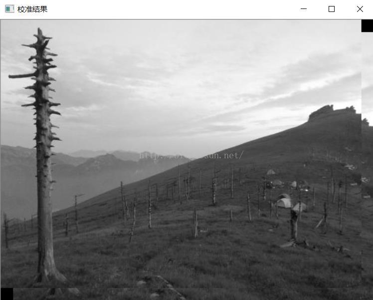
- imshow("校准结果", dst);
-
- waitKey(0);
- return 0;
- }
注意:最后的匹配结果保存在vector<DMatch>中。DMatch用来保存匹配后的结果
- struct DMatch
- {
- DMatch() :
- queryIdx(-1), trainIdx(-1), imgIdx(-1), distance(std::numeric_limits<float>::max()) {}
- DMatch(int _queryIdx, int _trainIdx, float _distance) :
- queryIdx(_queryIdx), trainIdx(_trainIdx), imgIdx(-1), distance(_distance) {}
- DMatch(int _queryIdx, int _trainIdx, int _imgIdx, float _distance) : queryIdx(_queryIdx), trainIdx(_trainIdx), imgIdx(_imgIdx), distance(_distance) {}
- int queryIdx;
- int trainIdx;
- int imgIdx;
- float distance;
- bool operator < (const DMatch &m) const;
- };
该校准结果是对上面这幅图中右边这幅偏移图像的校准结果,但是明显的问题是,边界问题没有处理好。
博文收录于转载:
一,图像配准算法小总结
首先,图像配准要素结合:特征空间,搜索空间,搜索策略,近似性度量;图像配准方法:
1.基于灰度信息的方法:交叉相关(互相关)方法,相关系数度量,序贯相似检测算法,信息理论的交换信息相似性准则。
2.基于变换域的方法:相位相关法,Walsh Transform变换。
3.基于特征的方法:常用的图像特征有:特征点(包括角点、高曲率点等)、直线段、边缘(Robert、高斯-拉普拉斯LoG、Canny、Gabor滤波等边缘检测算子)或轮廓、闭合区域、特征结构以及统计特征如矩不变量等。
注:像素灰度信息的互相关算法相比,特征提取包含了高层信号信息,所以该类算法对光照、噪声等的抗干扰能力强。
常用的空间变换模型:刚体变换(平移、旋转与缩放的组合)、仿射变换、透射变换、投影变换、非线性变换。
常用的相似性测度:
1.距离测度:均方根误差,差绝对值和误差,兰氏距离,Mahalanobis距离,绝对差,Hausdorff距离等。
2.角度度量法(概率测度)。
3.相关度量法
配准算法的评价标准:
配准时间、配准率、算法复杂度、算法的可移植性、算法的适用性、图像数据对算法的影响等(这里虽然不是目标追踪的评价标准,但是我们可以借鉴这些评价算法的标准)
二,图像配准算法分类
图像拼接技术主要包括两个关键环节即图像配准和图像融合对于图像融合部分,由于其耗时不太大,且现有的几种主要方法效果差别也不多,所以总体来说算法上比较成熟。而图像配准部分是整个图像拼接技术的核心部分,它直接关系到图像拼接算法的成功率和运行速度,因此配准算法的研究是多年来研究的重点。
目前的图像配准算法基本上可以分为两类:基于频域的方法(相位相关方法)和基于时域的方法。
相位相关法最早是由Kuglin和Hines在1975年提出的,并且证明在纯二维平移的情形下,拼接精度可以达到1个像素,多用于航空照片和卫星遥感图像的配准等领域。该方法对拼接的图像进行快速傅立叶变换,将两幅待配准图像变换到频域,然后通过它们的互功率谱直接计算出两幅图像间的平移矢量,从而实现图像的配准。由于其具有简单而精确的特点,后来成为最有前途的图像配准算法之一。但是相位相关方法一般需要比较大的重叠比例(通常要求配准图像之间有50%的重叠比例),如果重叠比例较小,则容易造成平移矢量的错误估计,从而较难实现图像的配准。
基于时域的方法又可具体分为基于特征的方法和基于区域的方法。基于特征的方法首先找出两幅图像中的特征点(如边界点、拐点),并确定图像间特征点的对应关系,然后利用这种对应关系找到两幅图像间的变换关系。这一类方法不直接利用图像的灰度信息,因而对光线变化不敏感,但对特征点对应关系的精确程度依赖很大。这一类方法采用的思想较为直观,目前大部分的图像配准算法都可以归为这一类。基于区域的方法是以一幅图像重叠区域中的一块作为模板,在另一幅图像中搜索与此模板最相似的匹配块,这种算法精度较高,但计算量过大。
按照匹配算法的具体实现又可以分为直接法和搜索法两大类,直接法主要包括变换优化法,它首先建立两幅待拼接图像间的变换模型,然后采用非线性迭代最小化算法直接计算出模型的变换参数,从而确定图像的配准位置。该算法效果较好,收敛速度较快,但是它要达到过程的收敛要求有较好的初始估计,如果初始估计不好,则会造成图像拼接的失败。搜索法主要是以一幅图像中的某些特征为依据,在另一幅图像中搜索最佳配准位置,常用的有比值匹配法,块匹配法和网格匹配法。比值匹配法是从一幅图像的重叠区域中部分相邻的两列上取出部分像素,然后以它们的比值作模板,在另一幅图像中搜索最佳匹配。这种算法计算量较小,但精度较低;块匹配法则是以一幅图像重叠区域中的一块作为模板,在另一幅图像中搜索与此模板最相似的匹配块,这种算法精度较高,但计算量过大;网格匹配法减小了块匹配法的计算量,它首先要进行粗匹配,每次水平或垂直移动一个步长,记录最佳匹配位置,然后在此位置附近进行精确匹配,每次步长减半,然后循环此过程直至步长减为0。这种算法较前两种运算量都有所减小,但在实际应用中仍然偏大,而且粗匹配时如果步长取的太大,很可能会造成较大的粗匹配误差,从而很难实现精确匹配。
参考资源:
【1】http://blog.csdn.net/zddblog/article/details/7521424
【2】http://www.cs.ubc.ca/~lowe/keypoints/
【3】http://blog.csdn.net/zhaocj/article/details/42124473
【4】http://www.cnblogs.com/cj695/p/4041478.html
【5】http://blog.csdn.net/llw01/article/details/9258699
【6】http://blog.csdn.net/xuluohongshang/article/details/52886352
注:本博文为EbowTang原创,后续可能继续更新本文。如果转载,请务必复制本条信息!
原文地址:http://blog.csdn.net/ebowtang/article/details/51236061
原作者博客:http://blog.csdn.net/ebowtang
版权声明:本文为EbowTang原创文章,后续可能继续更新本文。如果转载,请务必复制本文末尾的信息!


 895
895

 被折叠的 条评论
为什么被折叠?
被折叠的 条评论
为什么被折叠?
 到【灌水乐园】发言


