excel一键切换图表_一键创建Excel图表

excel一键切换图表

Did you know that it only takes one keystroke to create a chart from data in Excel? Here are the simple steps to create a very quick Excel chart.

您知道吗，只需一次按键即可从Excel中的数据创建图表？ 这是创建非常快速的Excel图表的简单步骤。

• First, select a cell that contains the chart data, or select a heading in one of the data rows or columns
  首先，选择一个包含图表数据的单元格，或者在数据行或列之一中选择标题

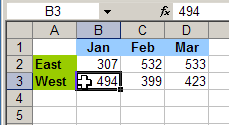
In the screen shot below, the data is in A1:D3, and cell B3 is selected.

在下面的屏幕快照中，数据在A1：D3中，并且选择了单元格B3。

NOTE: Cell A1, at the top left corner of the chart data is empty. That makes it easier for Excel to create a quick chart.

注意 ：图表数据左上角的单元格A1为空。 这使Excel可以更轻松地创建快速图表。

• Next, on the keyboard, press the F11 key

  接下来，在键盘上按F11键

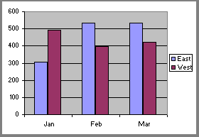
A chart sheet is inserted in the active workbook, with a chart in the default chart type, as shown below.

图表工作表将插入活动工作簿中，并且图表为默认图表类型，如下所示。

In the sample workbook, the default chart type is a Clustered Column. There are two columns for each month, with East in light purple, and West in dart purple..

在示例工作簿中，默认图表类型为“群集列”。 每个月有两栏，东为浅紫色，西为Dart紫色。

Just remember -- this is a super quick way to add a chart in Excel. After you insert that Excel chart so quickly, don't be tempted to spend another couple of hours playing with the formatting, to make it look perfect!

请记住-这是在Excel中添加图表的超快速方法。 在您如此Swift地插入Excel图表之后，请不要再花几个小时来处理格式，以使其看起来完美！

翻译自: https://contexturesblog.com/archives/2008/05/21/create-an-excel-chart-with-one-keystroke/

excel一键切换图表