使用切片器在Excel 2010中过滤表

最新推荐文章于 2022-05-27 11:41:32 发布

culiao2169

最新推荐文章于 2022-05-27 11:41:32 发布

阅读量433

点赞数

文章标签：过滤器 java vue excel python ViewUI

原文链接：https://contexturesblog.com/archives/2013/05/14/use-slicers-to-filter-a-table-in-excel-2010/

版权

Pivot table filtering was improved in Excel 2010, when Slicers were introduced. Instead of using the drop down lists in the pivot table headings, you can click on a Slicer, to quickly filter the pivot table. You couldn't use Slicers to filter a table in Excel 2010 though.

引入切片器后，Excel 2010中改进了数据透视表过滤。无需使用数据透视表标题中的下拉列表，您可以单击Slicer来快速筛选数据透视表。但是，您无法使用切片器在Excel 2010中过滤表。

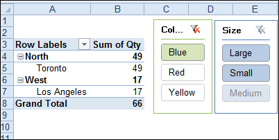
Slicers take up some room on the worksheet, but you can quickly see what filters have been applied. And, unlike Report Filters, Slicers show you what is available in the other fields, after you have applied a filter.

切片器在工作表上占据了一些空间，但是您可以快速查看已应用了哪些过滤器。而且，与报告过滤器不同，切片器会在应用过滤器后向您显示其他字段中的可用内容。

Excel表切片器 (Slicers for Excel Tables)

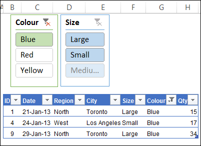
In Excel 2013, Slicers were enabled for named tables too, so you can filter your data with a single click. They work just like Pivot Table Slicers, and are especially handy if you’re doing a presentation. You can click one of the big Slicer buttons, instead of fumbling through the filter drop downs.

在Excel 2013中，也为命名表启用了切片器，因此您只需单击即可过滤数据。它们的工作方式与数据透视表切片器一样，如果要进行演示，则特别方便。您可以单击“切片器”大按钮之一，而不必在过滤器下拉菜单中进行任何操作。

Excel 2010表格的解决方法 (Workaround for Excel 2010 Tables)

Slicers don’t work on Excel 2010 tables, but if you’re using that version, there’s good news – AlexJ has developed a workaround.

切片器不适用于Excel 2010表格，但如果您使用的是该版本，则有个好消息– AlexJ已开发出一种解决方法。

There are a couple of limitations:

有两个限制：

You need a unique identifier in each table row.
每个表行中都需要一个唯一的标识符。
Changes made manually to the field filters on the table are not reflected on the slicers (you might want to hide the table filters)
手动对表中的字段过滤器进行的更改不会反映在切片器上(您可能希望隐藏表过滤器 )

添加数据透视表和切片器 (Add a Pivot Table and Slicers)

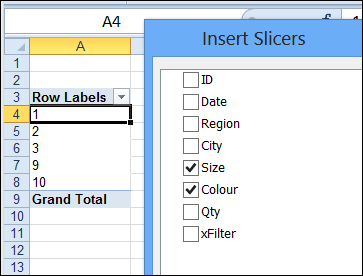
From the Excel table’s data, AlexJ built a pivot table, with the ID field in the Row Labels area. Next, he added two Slicers for the pivot table, using the Size and Colour fields.

AlexJ从Excel表的数据中构建了一个数据透视表，其中ID字段位于“行标签”区域中。接下来，他使用“大小”和“颜色”字段为数据透视表添加了两个“切片器”。

Then, copy or move those Slicers to the worksheet where the Excel Table is located.

然后，将那些“切片器”复制或移动到Excel表所在的工作表中。

检查ID (Check for the ID)

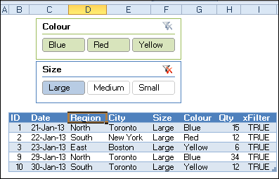
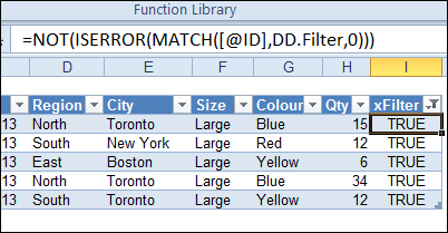
A named range – DD.Filter – is created, based on column A on the pivot table worksheet. In the Excel Table, a new column is added – xFilter – and a formula in that column checks for the row’s ID in the DD.Filter range.

基于数据透视表工作表上的列A，创建了一个命名范围DD.Filter。在Excel表中，添加了一个新列– xFilter –，该列中的公式将检查DD.Filter范围内的行ID。

The formula result is TRUE or FALSE, and only the TRUE rows will show after a Slicer is clicked.

公式结果为TRUE或FALSE，单击“切片器”后将仅显示TRUE行。

添加一些事件代码 (Add Some Event Code)

The final step is to add some event code to the pivot table, so it filters the table after a pivot table update. The pivot table update event is fired by the user action of changing a slicer selection.

最后一步是将一些事件代码添加到数据透视表中，以便在更新数据透视表后过滤该表。更改切片器选择的用户操作会触发数据透视表更新事件。

Here is the code from the SalesPivot worksheet module.

这是SalesPivot工作表模块中的代码。

Private Sub Worksheet_PivotTableUpdate(ByVal Target As PivotTable)
    Dim tbl As ListObject
    Dim lCol As Long
    Application.ScreenUpdating = False
    Set tbl = Worksheets("SalesData").ListObjects("Table1")
    lCol = tbl.ListColumns("xFilter").Index
    With tbl
        If .AutoFilter.FilterMode Then .AutoFilter.ShowAllData
        .Range.AutoFilter Field:=lCol, Criteria1:="TRUE"
    End With
    Application.ScreenUpdating = True
    Set tbl = Nothing
End Sub