在Excel 2010中过滤数据透视图

在Excel 2010中过滤数据透视图 (Filter Pivot Charts in Excel 2010)

In Excel 2007, there was a PivotChart Filter Pane, and you had to open that if you wanted to filter the pivot chart. Things have improved in Excel 2010, and the PivotChart Filter Pane is gone.

在Excel 2007中，有一个“数据透视图”过滤器窗格，如果要过滤数据透视图，则必须打开它。 Excel 2010中的情况有所改善，并且数据透视图筛选器窗格已消失。

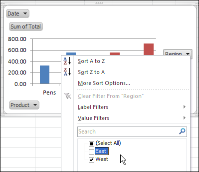
The field names now appear on the pivot chart, which is great news! Each field button has a drop down arrow, and you can use those drop downs to quickly and easily add or clear the filters.

字段名称现在出现在数据透视图上，这是个好消息！ 每个字段按钮都有一个下拉箭头，您可以使用这些下拉菜单快速轻松地添加或清除过滤器。

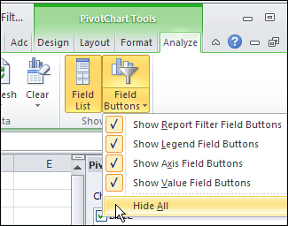
You can show or hide the individual field buttons, or use the Hide All command on the Ribbon, to control what appears in the pivot chart.

您可以显示或隐藏单个字段按钮，或使用功能区上的“全部隐藏”命令来控制数据透视表中显示的内容。

观看数据透视图过滤器视频 (Watch the Pivot Chart Filter Video)

To see the steps for creating and filtering a pivot chart in Excel 2010, you can watch this short Excel tutorial video.

若要查看在Excel 2010中创建和过滤数据透视图的步骤，您可以观看这段简短的Excel教程视频。

翻译自: https://contexturesblog.com/archives/2011/04/04/filter-pivot-charts-in-excel-2010/