epsg:欧洲石油调查组织_自组织地图：深入

epsg:欧洲石油调查组织

About David: David Asboth is a Data Scientist with a software development background. He’s had many different job titles over the years, with a common theme: he solves human problems with computers and data. This post originally appeared on his blog, davidasboth.com

关于David ：David Asboth是一位具有软件开发背景的数据科学家。 这些年来，他拥有许多不同的职位，并具有一个共同的主题：他用计算机和数据解决人为问题。 该帖子最初出现在他的博客davidasboth.com上

介绍 (Introduction)

In Part 1, I introduced the concept of Self-Organising Maps (SOMs). Now in Part 2 I want to step through the process of training and using a SOM – both the intuition and the Python code. At the end I’ll also present a couple of real life use cases, not just the toy example we’ll use for implementation.

在第1部分中 ，我介绍了自组织映射（SOM）的概念。 现在，在第2部分中，我想逐步训练和使用SOM的过程–直觉和Python代码。 最后，我还将介绍几个实际的用例，而不仅仅是我们将用于实现的玩具示例。

The first thing we need is a problem to solve!

我们需要做的第一件事就是解决问题！

I’ll use the colour map as the walkthrough example because it lends itself very nicely to visualisation.

我将使用颜色贴图作为演练示例，因为它非常适合可视化。

建立 (Setup)

数据集 (Dataset)

Our data will be a collection of random colours, so first we’ll artificially create a dataset of 100. Each colour is a 3D vector representing R, G and B values:

我们的数据将是随机颜色的集合，因此首先我们将人为创建100个数据集。每种颜色都是代表R，G和B值的3D矢量：

import numpy as np
raw_data = np.random.randint(0, 255, (3, 100))

import numpy as np
raw_data = np.random.randint(0, 255, (3, 100))

That’s simply 100 rows of 3D vectors all between the values of 0 and 255.

这就是100行3D向量，介于0和255之间。

目的 (Objective)

Just to be clear, here’s what we’re trying to do. We want to take our 3D colour vectors and map them onto a 2D surface in such a way that similar colours will end up in the same area of the 2D surface.

为了清楚起见，这是我们正在尝试做的事情。 我们要获取3D颜色矢量并将其映射到2D曲面上，以使相似的颜色最终出现在2D曲面的相同区域中。

SOM参数 (SOM Parameters)

Before training a SOM we need to decide on a few parameters.

在训练SOM之前，我们需要确定一些参数。

SOM尺寸 (SOM Size)

First of all, its dimensionality. In theory, a SOM can be any number of dimensions, but for visualisation purposes it is typically 2D and that’s what I’ll be using too.

首先，它的维度。 从理论上讲，SOM可以是任意数量的尺寸，但是出于可视化目的，它通常是2D的，这也是我将要使用的尺寸。

We also need to decide the number of neurons in the 2D grid. This is one of those decisions in machine learning that might as well be black magic, so we probably need to try a few sizes to get one that feels right.

我们还需要确定2D网格中神经元的数量。 这是机器学习中的决定之一，也可能是不可思议的，因此我们可能需要尝试一些尺寸才能获得合适的尺寸。

Remember, this is unsupervised learning, meaning whatever answer the algorithm comes up with will have to be evaluated somewhat subjectively. It’s typical in an unsupervised problem (e.g. k-means clustering) to do multiple runs and see what works.

请记住，这是无监督的学习，这意味着算法给出的任何答案都必须在主观上进行评估。 在无人监督的问题（例如，k均值聚类）中，进行多次运行并查看有效方法是很典型的。

I’ll go with a 5 by 5 grid. I guess one rule of thumb should be to use fewer neurons than you have data points, otherwise they might not overlap. As we’ll see we actually want them to overlap, because having multiple 3D vectors mapping to the same point in 2D is how we find similarities between our data points.

我将使用5 x 5网格。 我想一个经验法则是使用少于数据点的神经元，否则它们可能不会重叠。 正如我们将看到的，我们实际上希望它们重叠，因为有多个3D向量映射到2D中的同一点是我们发现数据点之间相似性的方式。

One important aspect of the SOM is that each of the 2D points on the grid actually represent a multi-dimensional weight vector. Each point on the SOM has a weight vector associated with it that is the same number of dimensions as our input data, in this case 3 to match the 3 dimensions of our colours. We’ll see why this is important when we go through the implementation.

SOM的一个重要方面是，网格上的每个2D点实际上代表一个多维权重向量。 SOM上的每个点都有一个与之关联的权重向量，该权重向量与我们的输入数据的维数相同，在这种情况下为3，以匹配我们的颜色的3维。 我们将在实施过程中了解为什么这很重要。

学习参数 (Learning Parameters)

Training the SOM is an iterative process – it will get better at its task with every iteration, so we need a cutoff point. Our problem is quite small so 2,000 iterations should suffice but in bigger problems it’s quite possible to need over 10,000.

培训SOM是一个反复的过程-它会在每次迭代中都变得更好，因此我们需要一个起点。 我们的问题很小，因此2,000次迭代就足够了，但是在更大的问题中，很有可能需要超过10,000次。

We also need a learning rate. The learning rate decides by how much we apply changes to our SOM at each iteration.

我们还需要学习率。 学习率取决于每次迭代对SOM应用多少更改。

If it’s too high, we will keep making drastic changes to the SOM and might never settle on a solution.

如果太高，我们将继续对SOM进行大幅度的更改，并且可能永远不会解决。

If it’s too low, we’ll never get anything done as we will only make very small changes.

如果它太低，我们将永远不会做任何事情，因为我们只会做很小的更改。

In practice it is best to start with a larger learning rate and reduce it slowly over time. This is so that the SOM can start by making big changes but then settle into a solution after a while.

在实践中，最好从更高的学习率开始，然后逐渐降低学习率。 这样，SOM可以先进行重大更改，然后过一会儿再解决。

实作 (Implementation)

For the rest of this post I will use 3D to refer to the dimensionality of the input data (which in reality could be any number of dimensions) and 2D as the dimensionality of the SOM (which we decide and could also be any number).

在本文的其余部分中，我将使用3D表示输入数据的维度（实际上可以是任意数量的维度），将2D称为SOM的维度（我们可以决定，也可以是任意数量）。

建立 (Setup)

To setup the SOM we need to start with the following:

要设置SOM，我们需要从以下内容开始：

• Decide on and initialise the SOM parameters (as above)
• Setup the grid by creating a 5×5 array of random 3D weight vectors

• 确定并初始化SOM参数（如上所述）
• 通过创建5×5随机3D权重向量的数组来设置网格

Those last two parameters relate to the 2D neighbourhood of each neuron in the SOM during training. We’ll return to those in the learning phase. Like the learning rate, the initial 2D radius will encompass most of the SOM and will gradually decrease as the number of iterations increases.

后两个参数与训练期间SOM中每个神经元的2D邻域有关。 我们将回到学习阶段。 像学习率一样，初始2D半径将包含大部分SOM，并且将随着迭代次数的增加而逐渐减小。

正常化 (Normalisation)

Another detail to discuss at this point is whether or not we normalise our dataset.

此时要讨论的另一个细节是是否对数据集进行规范化。

First of all, SOMs train faster (and “better”) if all our values are between 0 and 1. This is often true with machine learning problems, and it’s to avoid one of our dimensions “dominating” the others in the learning process. For example, if one of our variable was salary (in the thousands) and another was height (in metres, so rarely over 2.0) then salary will get a higher importance simply because it has much higher values. Normalising to the unit interval will remove this effect.

首先，如果我们所有的值都在0到1之间，那么SOM的训练速度就会更快（并且“更好”），这在机器学习问题中通常是正确的，并且是为了避免我们的一个维度在学习过程中“主导”其他维度。 例如，如果我们的变量之一是薪水（以千计），另一个是身高（以米为单位，所以很少超过2.0），那么薪水将具有更高的重要性，仅仅是因为它具有更高的价值。 归一化为单位间隔将消除此影响。

In our case all 3 dimensions refer to a value between 0 and 255 so we can normalise the entire dataset at once. However, if our variables were on different scales we would have to do this column by column.

在我们的案例中，所有3个维度均指的是介于0到255之间的值，因此我们可以一次将整个数据集标准化。 但是，如果变量的比例不同，则必须逐列进行。

I don’t want this code to be entirely tailored to the colour dataset so I’ll leave the normalisation options tied to a few Booleans that are easy to change.

我不希望此代码完全适合于颜色数据集，因此我将归一化选项与一些易于更改的布尔值联系在一起。

normalise_data = True

# if True, assume all data is on common scale
# if False, normalise to [0 1] range along each column
normalise_by_column = False

# we want to keep a copy of the raw data for later
data = raw_data

# check if data needs to be normalised
if normalise_data:
    if normalise_by_column:
        # normalise along each column
        col_maxes = raw_data.max(axis=0)
        data = raw_data / col_maxes[np.newaxis, :]
    else:
        # normalise entire dataset
        data = raw_data / data.max()

normalise_data = True

# if True, assume all data is on common scale
# if False, normalise to [0 1] range along each column
normalise_by_column = False

# we want to keep a copy of the raw data for later
data = raw_data

# check if data needs to be normalised
if normalise_data:
    if normalise_by_column:
        # normalise along each column
        col_maxes = raw_data.max(axis=0)
        data = raw_data / col_maxes[np.newaxis, :]
    else:
        # normalise entire dataset
        data = raw_data / data.max()

Now we’re ready to start the learning process.

现在我们准备开始学习过程。

学习 (Learning)

In broad terms the learning process will be as follows. We’ll fill in the implementation details as we go along.

概括地说，学习过程如下。 继续进行时，我们将填写实施细节。

For a single iteration:

对于一次迭代：

• Find the neuron in the SOM whose associated 3D vector is closest to our chosen 3D colour vector. At each step, this is called the Best Matching Unit (BMU)
• Move the BMU’s 3D weight vector closer to the input vector in 3D space
• Identify the 2D neighbours of the BMU and also move their 3D weight vectors closer to the input vector, although by a smaller amount
• Update the learning rate (reduce it at each iteration)

• 在SOM中找到其关联的3D向量最接近我们选择的3D颜色向量的神经元。 在每个步骤中，这都称为最佳匹配单元（BMU）
• 将BMU的3D权重向量移到3D空间中的输入向量附近
• 识别BMU的2D邻居，并将其3D权重向量移近输入向量，尽管数量较小
• 更新学习率（每次迭代降低学习率）

And that’s it. By doing the penultimate step, moving the BMU’s neighbours, we’ll achieve the desired effect that colours that are close in 3D space will be mapped to similar areas in 2D space.

就是这样。 通过执行倒数第二步，移动BMU的邻居，我们将达到预期的效果，即3D空间中接近的颜色将被映射到2D空间中的相似区域。

Let’s step through this in more detail, with code.

让我们通过代码来更详细地逐步介绍。

1.选择一个随机输入向量 (1. Select a Random Input Vector)

This is straightforward:

这很简单：

2.找到最佳匹配单位 (2. Find the Best Matching Unit)

# find its Best Matching Unit
bmu, bmu_idx = find_bmu(t, net, m)

# find its Best Matching Unit
bmu, bmu_idx = find_bmu(t, net, m)

For that to work we need a function to find the BMU. It need to iterate through each neuron in the SOM, measure its Euclidean distance to our input vector and return the one that’s closest. Note the implementation trick of not actually measuring Euclidean distance, but the squared Euclidean distance, thereby avoiding an expensive square root computation.

为此，我们需要一个函数来查找BMU。 它需要遍历SOM中的每个神经元，测量其到我们输入向量的欧几里得距离，并返回最接近的一个。 注意，实现技巧不是实际测量欧几里得距离，而是平方欧几里德距离，从而避免了昂贵的平方根计算。

3.更新SOM学习参数 (3. Update the SOM Learning Parameters)

As described above, we want to decay the learning rate over time to let the SOM “settle” on a solution.

如上所述，我们希望随着时间的推移降低学习率，以使SOM能够“解决”解决方案。

What we also decay is the neighbourhood radius, which defines how far we search for 2D neighbours when updating vectors in the SOM. We want to gradually reduce this over time, like the learning rate. We’ll see this in a bit more detail in step 4.

我们还要衰减的是邻域半径，它定义了更新SOM中的向量时搜索2D邻居的距离。 我们希望随着学习时间的增长逐渐减少这种情况。 我们将在步骤4中看到更多细节。

# decay the SOM parameters
r = decay_radius(init_radius, i, time_constant)
l = decay_learning_rate(init_learning_rate, i, n_iterations)

# decay the SOM parameters
r = decay_radius(init_radius, i, time_constant)
l = decay_learning_rate(init_learning_rate, i, n_iterations)

The functions to decay the radius and learning rate use exponential decay:

衰减半径和学习率的函数使用指数衰减：

Where $lambda$ is the time constant (which controls the decay) and $sigma$ is the value at various times $t$.

其中$ lambda $是时间常数（控制衰减），而$ sigma $是在不同时间$ t $的值。

3.在3D空间中移动BMU及其邻居 (3. Move the BMU and its Neighbours in 3D Space)

Now that we have the BMU and the correct learning parameters, we’ll update the SOM so that this BMU is now closer in 3D space to the colour that mapped to it. We will also identify the neurons that are close to the BMU in 2D space and update their 3D vectors to move “inwards” towards the BMU.

现在我们有了BMU和正确的学习参数，我们将更新SOM，以便此BMU现在在3D空间中更接近映射到它的颜色。 我们还将识别2D空间中靠近BMU的神经元，并更新其3D向量以向内向BMU移动。

The formula to update the BMU’s 3D vector is:

更新BMU 3D向量的公式为：

That is to say, the new weight vector will be the current vector plus the difference between the input vector $V$ and the weight vector, multiplied by a learning rate $L$ at time $t$.

也就是说，新的权重向量将是当前向量加上输入向量$ V $和权重向量之间的差，再乘以时间$ t $的学习率$ L $。

We are literally just moving the weight vector closer to the input vector.

实际上，我们只是将权重向量移近输入向量。

We also identify all the neurons in the SOM that are closer in 2D space than our current radius, and also move them closer to the input vector.

我们还确定了SOM中在2D空间中比我们当前半径更近的所有神经元，并将它们移近了输入向量。

The difference is that the weight update will be proportional to their 2D distance from the BMU.

不同之处在于权重更新将与其距BMU的2D距离成正比。

One last thing to note: this proportion of 2D distance isn’t uniform, it’s Gaussian. So imagine a bell shape centred around the BMU – that’s how we decide how much to pull the neighbouring neurons in by.

最后要注意的一件事：2D距离的比例不是均匀的，是高斯。 因此，想象一下以BMU为中心的钟形形状-这就是我们决定拉近相邻神经元的程度的方式。

Concretely, this is the equation we’ll use to calculate the influence $i$:

具体来说，这是我们用来计算影响力$ i $的方程式：

where $d$ is the 2D distance and $sigma$ is the current radius of our neighbourhood.

其中$ d $是2D距离，而$ sigma $是我们附近的当前半径。

Putting that all together:

放在一起：

def calculate_influence(distance, radius):
    return np.exp(-distance / (2* (radius**2))

# now we know the BMU, update its weight vector to move closer to input
# and move its neighbours in 2-D space closer
# by a factor proportional to their 2-D distance from the BMU
for x in range(net.shape[0]):
    for y in range(net.shape[1]):
        w = net[x, y, :].reshape(m, 1)
        # get the 2-D distance (again, not the actual Euclidean distance)
        w_dist = np.sum((np.array([x, y]) - bmu_idx) ** 2)
        # if the distance is within the current neighbourhood radius
        if w_dist <= r**2:
            # calculate the degree of influence (based on the 2-D distance)
            influence = calculate_influence(w_dist, r)
            # now update the neuron's weight using the formula:
            # new w = old w + (learning rate * influence * delta)
            # where delta = input vector (t) - old w
            new_w = w + (l * influence * (t - w))
            # commit the new weight
            net[x, y, :] = new_w.reshape(1, 3)

def calculate_influence(distance, radius):
    return np.exp(-distance / (2* (radius**2))

# now we know the BMU, update its weight vector to move closer to input
# and move its neighbours in 2-D space closer
# by a factor proportional to their 2-D distance from the BMU
for x in range(net.shape[0]):
    for y in range(net.shape[1]):
        w = net[x, y, :].reshape(m, 1)
        # get the 2-D distance (again, not the actual Euclidean distance)
        w_dist = np.sum((np.array([x, y]) - bmu_idx) ** 2)
        # if the distance is within the current neighbourhood radius
        if w_dist <= r**2:
            # calculate the degree of influence (based on the 2-D distance)
            influence = calculate_influence(w_dist, r)
            # now update the neuron's weight using the formula:
            # new w = old w + (learning rate * influence * delta)
            # where delta = input vector (t) - old w
            new_w = w + (l * influence * (t - w))
            # commit the new weight
            net[x, y, :] = new_w.reshape(1, 3)

可视化 (Visualization)

Repeating the learning steps 1-4 for 2,000 iterations should be enough. We can always run it for more iterations afterwards.

重复学习步骤1-4 2,000次迭代就足够了。 之后，我们总是可以对其进行更多迭代。

Handily, the 3D weight vectors in the SOM can also be interpreted as colours, since they are just 3D vectors just like the inputs.

方便地，SOM中的3D权向量也可以解释为颜色，因为它们就像输入一样只是3D向量。

To that end, we can visualise them and come up with our final colour map:

为此，我们可以对其可视化，并得出最终的颜色图：

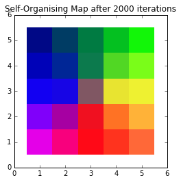
A self-organising colour map

自组织的颜色图

None of those colours necessarily had to be in our dataset. By moving the 3D weight vectors to more closely match our input vectors, we’ve created a 2D colour space which clearly shows the relationship between colours. More blue colours will map to the left part of the SOM, whereas reddish colours will map to the bottom, and so on.

这些颜色都不必一定在我们的数据集中。 通过移动3D权重向量以使其更接近我们的输入向量，我们创建了2D颜色空间，该空间清楚地显示了颜色之间的关系。 更多的蓝色将映射到SOM的左侧，而红色将映射到底部，依此类推。

其他例子 (Other Examples)

Finding a 2D colour space is a good visual way to get used to the idea of a SOM. However, there are obviously practical applications of this algorithm.

找到2D色彩空间是习惯SOM想法的一种很好的视觉方法。 但是，显然有该算法的实际应用。

虹膜数据集 (Iris Dataset)

A dataset favoured by the machine learning community is Sir Ronald Fisher’s dataset of measurements of irises. There are four input dimensions: petal width, petal length, sepal width and sepal length and we could use a SOM to find similar flowers.

机器学习社区青睐的数据集是Ronald Fisher爵士的虹膜测量数据集 。 输入有四个维度：花瓣宽度，花瓣长度，萼片宽度和萼片长度，我们可以使用SOM查找相似的花朵。

Applying the iris data to a SOM and then retrospectively colouring each point with their true class (to see how good the SOM was at separating the irises into their distinct categories) we get something like this:

将虹膜数据应用于SOM，然后使用真实类对每个点进行回顾性着色（以查看SOM在将虹膜分为不同类别方面的表现如何），我们得到以下信息：

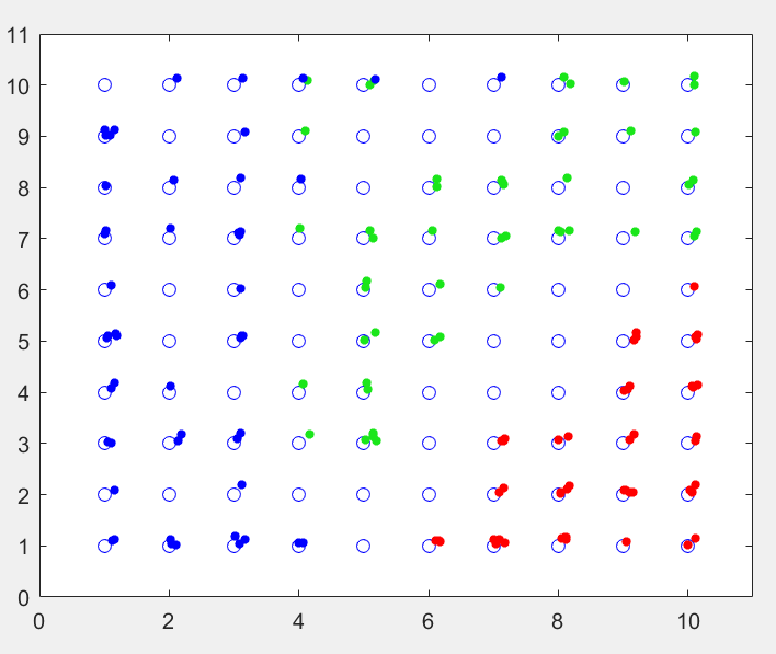
150 irises mapped onto a SOM, coloured by type

将150个光圈映射到SOM，按类型上色

This is a 10 by 10 SOM and each of the small points is one of the irises from the dataset (with added jitter to see multiple points on a single SOM neuron). I added the colours after training, and you can quite clearly see the 3 distinct regions the SOM has divided itself into.

这是一个10 x 10的SOM，每个小点都是数据集中的虹膜之一（增加了抖动以查看单个SOM神经元上的多个点）。 我在训练后添加了颜色，您可以很清楚地看到SOM划分为3个不同的区域。

There are a few SOM neurons where both the green and the blue points get assigned to, and this represents the overlap between the versicolor and virginica types.

在绿色和蓝色点都分配了一些SOM神经元的情况下，这表示杂色和弗吉尼亚类型之间的重叠。

手写数字 (Handwritten Digits)

Another application I touched on in Part 1 is trying to identify handwritten characters.

我在第1部分中涉及的另一个应用程序正在尝试识别手写字符。

In this case, the inputs are high-dimensional – each input dimension represents the grayscale value of one pixel on a 28 by 28 image. That makes the inputs 784-dimensional (each dimension is a value between 0 and 255).

在这种情况下，输入为高维-每个输入维代表28 x 28图像上一个像素的灰度值。 这使输入为784维（每个维是介于0到255之间的值）。

Mapping them to a 20 by 20 SOM, and again retrospectively colouring them based on their true class (a number from 0 to 9) yields this:

将它们映射到20 x 20的SOM，然后再次根据其真实类（从0到9的数字）为它们着色：

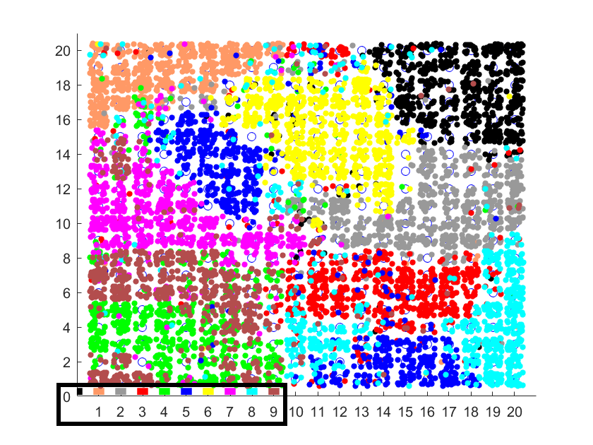
Various handwritten numbers mapped to a 2D SOM

各种手写数字映射到2D SOM

In this case the true classes are labelled according to the colours in the bottom left.

在这种情况下，根据左下角的颜色标记真实的类。

What you can see is that the SOM has successfully divided the 2D space into regions. Despite some overlap, in most cases similar digits get mapped to the same region.

您会看到，SOM已成功将2D空间划分为多个区域。 尽管有一些重叠，但在大多数情况下，相似的数字会映射到相同的区域。

For example, the yellow region is where the 6s were mapped, and there is little overlap with other categories. Whereas in the bottom left, where the green and brown points overlap, is where the SOM was “confused” between 4s and 9s. A visual inspection of some of these handwritten characters shows that indeed many of the 4s and 9s are easily confused.

例如，黄色区域是6s的映射位置，与其他类别几乎没有重叠。 而在左下角（绿色和棕色点重叠）是SOM在4s和9s之间“混淆”的地方。 对这些手写字符中的某些手写字符进行目视检查后发现，确实很容易混淆4s和9s中的许多字符。

进一步阅读 (Further Reading)

翻译自: https://www.pybloggers.com/2017/03/self-organising-maps-in-depth/

epsg:欧洲石油调查组织