带有Python的AI –监督学习：分类

最新推荐文章于 2023-07-01 16:44:05 发布

cunzai1985

最新推荐文章于 2023-07-01 16:44:05 发布

阅读量869

点赞数 2

文章标签：决策树 python 机器学习人工智能深度学习

原文链接：https://www.tutorialspoint.com/artificial_intelligence_with_python/artificial_intelligence_with_python_supervised_learning_classification.htm

版权

带有Python的AI –监督学习：分类 (AI with Python – Supervised Learning: Classification)

In this chapter, we will focus on implementing supervised learning − classification.

在本章中，我们将重点介绍实施监督学习-分类。

The classification technique or model attempts to get some conclusion from observed values. In classification problem, we have the categorized output such as “Black” or “white” or “Teaching” and “Non-Teaching”. While building the classification model, we need to have training dataset that contains data points and the corresponding labels. For example, if we want to check whether the image is of a car or not. For checking this, we will build a training dataset having the two classes related to “car” and “no car”. Then we need to train the model by using the training samples. The classification models are mainly used in face recognition, spam identification, etc.

分类技术或模型试图从观测值中得出一些结论。在分类问题中，我们有分类输出，例如“黑色”或“白色”或“示教”和“非示教”。在建立分类模型时，我们需要具有包含数据点和相应标签的训练数据集。例如，如果我们要检查图像是否是汽车。为了进行检查，我们将构建一个训练数据集，其中包含与“汽车”和“无汽车”相关的两个类别。然后，我们需要使用训练样本来训练模型。分类模型主要用于人脸识别，垃圾邮件识别等。

在Python中构建分类器的步骤 (Steps for Building a Classifier in Python)

For building a classifier in Python, we are going to use Python 3 and Scikit-learn which is a tool for machine learning. Follow these steps to build a classifier in Python −

为了在Python中构建分类器，我们将使用Python 3和Scikit-learn(这是一种用于机器学习的工具)。请按照以下步骤在Python中构建分类器-

第1步-导入Scikit学习 (Step 1 − Import Scikit-learn)

This would be very first step for building a classifier in Python. In this step, we will install a Python package called Scikit-learn which is one of the best machine learning modules in Python. The following command will help us import the package −

这将是在Python中构建分类器的第一步。在这一步中，我们将安装一个名为Scikit-learn的Python包，它是Python中最好的机器学习模块之一。以下命令将帮助我们导入包-


Import Sklearn

第2步-导入Scikit-learn的数据集 (Step 2 − Import Scikit-learn’s dataset)

In this step, we can begin working with the dataset for our machine learning model. Here, we are going to use the Breast Cancer Wisconsin Diagnostic Database. The dataset includes various information about breast cancer tumors, as well as classification labels of malignant or benign. The dataset has 569 instances, or data, on 569 tumors and includes information on 30 attributes, or features, such as the radius of the tumor, texture, smoothness, and area. With the help of the following command, we can import the Scikit-learn’s breast cancer dataset −

在这一步中，我们可以开始使用机器学习模型的数据集。在这里，我们将要使用的乳腺癌诊断威斯康星数据库。该数据集包括有关乳腺癌肿瘤的各种信息，以及恶性或良性的分类标签。该数据集包含569个肿瘤的569个实例或数据，并包含有关30个属性或特征的信息，例如肿瘤的半径，纹理，光滑度和面积。借助以下命令，我们可以导入Scikit-learn的乳腺癌数据集-


from sklearn.datasets import load_breast_cancer

Now, the following command will load the dataset.

现在，以下命令将加载数据集。


data = load_breast_cancer()

Following is a list of important dictionary keys −

以下是重要的字典键列表-

Classification label names(target_names)
分类标签名称(target_names)
The actual labels(target)
实际标签(目标)
The attribute/feature names(feature_names)
属性/功能名称(feature_names)
The attribute (data)
属性(数据)

Now, with the help of the following command, we can create new variables for each important set of information and assign the data. In other words, we can organize the data with the following commands −

现在，借助以下命令，我们可以为每组重要信息创建新变量并分配数据。换句话说，我们可以使用以下命令来组织数据-


label_names = data['target_names']
labels = data['target']
feature_names = data['feature_names']
features = data['data']

Now, to make it clearer we can print the class labels, the first data instance’s label, our feature names and the feature’s value with the help of the following commands −

现在，为了更清楚一点，我们可以在以下命令的帮助下打印类标签，第一个数据实例的标签，功能名称和功能值-


print(label_names)

The above command will print the class names which are malignant and benign respectively. It is shown as the output below −

上面的命令将分别打印恶性和良性的类名。它显示为下面的输出-


['malignant' 'benign']

Now, the command below will show that they are mapped to binary values 0 and 1. Here 0 represents malignant cancer and 1 represents benign cancer. You will receive the following output −

现在，下面的命令将显示它们已映射到二进制值0和1。这里0表示恶性癌症，而1表示良性癌症。您将收到以下输出-


print(labels[0])
0

The two commands given below will produce the feature names and feature values.

下面给出的两个命令将生成要素名称和要素值。


print(feature_names[0])
mean radius
print(features[0])
[ 1.79900000e+01 1.03800000e+01 1.22800000e+02 1.00100000e+03
  1.18400000e-01 2.77600000e-01 3.00100000e-01 1.47100000e-01
  2.41900000e-01 7.87100000e-02 1.09500000e+00 9.05300000e-01
  8.58900000e+00 1.53400000e+02 6.39900000e-03 4.90400000e-02
  5.37300000e-02 1.58700000e-02 3.00300000e-02 6.19300000e-03
  2.53800000e+01 1.73300000e+01 1.84600000e+02 2.01900000e+03
  1.62200000e-01 6.65600000e-01 7.11900000e-01 2.65400000e-01
  4.60100000e-01 1.18900000e-01]

From the above output, we can see that the first data instance is a malignant tumor the radius of which is 1.7990000e+01.

从上面的输出中，我们可以看到第一个数据实例是一个恶性肿瘤，其半径为1.7990000e + 01。

第3步-将数据组织成组 (Step 3 − Organizing data into sets)

In this step, we will divide our data into two parts namely a training set and a test set. Splitting the data into these sets is very important because we have to test our model on the unseen data. To split the data into sets, sklearn has a function called the train_test_split() function. With the help of the following commands, we can split the data in these sets −

在这一步中，我们将数据分为训练集和测试集两部分。将数据分为这些集合非常重要，因为我们必须在看不见的数据上测试模型。为了将数据分成几组，sklearn具有一个称为train_test_split()函数的函数。借助以下命令，我们可以将数据拆分为以下几组：


from sklearn.model_selection import train_test_split

The above command will import the train_test_split function from sklearn and the command below will split the data into training and test data. In the example given below, we are using 40 % of the data for testing and the remaining data would be used for training the model.

上面的命令将从sklearn导入train_test_split函数，下面的命令将数据分为训练和测试数据。在下面给出的示例中，我们将40％的数据用于测试，其余数据将用于训练模型。


train, test, train_labels, test_labels = train_test_split(features,labels,test_size = 0.40, random_state = 42)

第4步-建立模型 (Step 4 − Building the model)

In this step, we will be building our model. We are going to use Naïve Bayes algorithm for building the model. Following commands can be used to build the model −

在此步骤中，我们将构建模型。我们将使用朴素贝叶斯算法来构建模型。以下命令可用于构建模型-


from sklearn.naive_bayes import GaussianNB

The above command will import the GaussianNB module. Now, the following command will help you initialize the model.

上面的命令将导入GaussianNB模块。现在，以下命令将帮助您初始化模型。


gnb = GaussianNB()

We will train the model by fitting it to the data by using gnb.fit().

我们将使用gnb.fit()将模型拟合到数据中来训练模型。


model = gnb.fit(train, train_labels)

步骤5-评估模型及其准确性 (Step 5 − Evaluating the model and its accuracy)

In this step, we are going to evaluate the model by making predictions on our test data. Then we will find out its accuracy also. For making predictions, we will use the predict() function. The following command will help you do this −

在这一步中，我们将通过对测试数据进行预测来评估模型。然后，我们还将找出其准确性。为了进行预测，我们将使用predict()函数。以下命令将帮助您做到这一点-


preds = gnb.predict(test)
print(preds)

[1 0 0 1 1 0 0 0 1 1 1 0 1 0 1 0 1 1 1 0 1 1 0 1 1 1 1 1 1
 0 1 1 1 1 1 1 0 1 0 1 1 0 1 1 1 1 1 1 1 1 0 0 1 1 1 1 1 0 
 0 1 1 0 0 1 1 1 0 0 1 1 0 0 1 0 1 1 1 1 1 1 0 1 1 0 0 0 0 
 0 1 1 1 1 1 1 1 1 0 0 1 0 0 1 0 0 1 1 1 0 1 1 0 1 1 0 0 0 
 1 1 1 0 0 1 1 0 1 0 0 1 1 0 0 0 1 1 1 0 1 1 0 0 1 0 1 1 0 
 1 0 0 1 1 1 1 1 1 1 0 0 1 1 1 1 1 1 1 1 1 1 1 1 0 1 1 1 0 
 1 1 0 1 1 1 1 1 1 0 0 0 1 1 0 1 0 1 1 1 1 0 1 1 0 1 1 1 0 
 1 0 0 1 1 1 1 1 1 1 1 0 1 1 1 1 1 0 1 0 0 1 1 0 1]

The above series of 0s and 1s are the predicted values for the tumor classes – malignant and benign.

上面的0和1系列是肿瘤类别(恶性和良性)的预测值。

Now, by comparing the two arrays namely test_labels and preds, we can find out the accuracy of our model. We are going to use the accuracy_score() function to determine the accuracy. Consider the following command for this −

现在，通过比较两个数组test_labels和preds ，我们可以找到模型的准确性。我们将使用precision_score()函数确定准确性。考虑以下命令-


from sklearn.metrics import accuracy_score
print(accuracy_score(test_labels,preds))
0.951754385965

The result shows that the NaïveBayes classifier is 95.17% accurate.

结果表明，NaïveBayes分类器的准确度为95.17％。

In this way, with the help of the above steps we can build our classifier in Python.

这样，借助以上步骤，我们可以在Python中构建分类器。

用Python构建分类器 (Building Classifier in Python)

In this section, we will learn how to build a classifier in Python.

在本节中，我们将学习如何在Python中构建分类器。

朴素贝叶斯分类器 (Naïve Bayes Classifier)

Naïve Bayes is a classification technique used to build classifier using the Bayes theorem. The assumption is that the predictors are independent. In simple words, it assumes that the presence of a particular feature in a class is unrelated to the presence of any other feature. For building Naïve Bayes classifier we need to use the python library called scikit learn. There are three types of Naïve Bayes models named Gaussian, Multinomial and Bernoulli under scikit learn package.

朴素贝叶斯是一种分类技术，用于使用贝叶斯定理构建分类器。假设是预测变量是独立的。简而言之，它假定类中某个特定功能的存在与任何其他功能的存在无关。为了构建朴素贝叶斯分类器，我们需要使用名为scikit learning的python库。在scikit学习包下，有三种类型的朴素贝叶斯模型分别称为Gaussian，Multinomial和Bernoulli 。

To build a Naïve Bayes machine learning classifier model, we need the following &minus

要建立朴素贝叶斯机器学习分类器模型，我们需要满足以下条件

数据集 (Dataset)

We are going to use the dataset named Breast Cancer Wisconsin Diagnostic Database. The dataset includes various information about breast cancer tumors, as well as classification labels of malignant or benign. The dataset has 569 instances, or data, on 569 tumors and includes information on 30 attributes, or features, such as the radius of the tumor, texture, smoothness, and area. We can import this dataset from sklearn package.

我们将使用名为乳腺癌威斯康星州诊断数据库的数据集。该数据集包括有关乳腺癌肿瘤的各种信息，以及恶性或良性的分类标签。该数据集包含569个肿瘤的569个实例或数据，并包含有关30个属性或特征的信息，例如肿瘤的半径，纹理，光滑度和面积。我们可以从sklearn包中导入该数据集。

朴素贝叶斯模型 (Naïve Bayes Model)

For building Naïve Bayes classifier, we need a Naïve Bayes model. As told earlier, there are three types of Naïve Bayes models named Gaussian, Multinomial and Bernoulli under scikit learn package. Here, in the following example we are going to use the Gaussian Naïve Bayes model.

为了构建朴素贝叶斯分类器，我们需要一个朴素贝叶斯模型。如前所述，在scikit学习包下，有三种类型的朴素贝叶斯模型分别称为高斯，多项式和伯努利 。在下面的示例中，我们将使用高斯朴素贝叶斯模型。

By using the above, we are going to build a Naïve Bayes machine learning model to use the tumor information to predict whether or not a tumor is malignant or benign.

通过使用以上内容，我们将建立一个朴素的贝叶斯机器学习模型，以使用肿瘤信息来预测肿瘤是恶性还是良性。

To begin with, we need to install the sklearn module. It can be done with the help of the following command −

首先，我们需要安装sklearn模块。可以在以下命令的帮助下完成-


Import Sklearn

Now, we need to import the dataset named Breast Cancer Wisconsin Diagnostic Database.

现在，我们需要导入名为乳腺癌威斯康星州诊断数据库的数据集。


from sklearn.datasets import load_breast_cancer

Now, the following command will load the dataset.

现在，以下命令将加载数据集。


data = load_breast_cancer()

The data can be organized as follows −

数据可以组织如下-


label_names = data['target_names']
labels = data['target']
feature_names = data['feature_names']
features = data['data']

Now, to make it clearer we can print the class labels, the first data instance’s label, our feature names and the feature’s value with the help of following commands −

现在，为了更清楚一点，我们可以在以下命令的帮助下打印类标签，第一个数据实例的标签，功能名称和功能值-


print(label_names)

The above command will print the class names which are malignant and benign respectively. It is shown as the output below −

上面的命令将分别打印恶性和良性的类名。它显示为下面的输出-


['malignant' 'benign']

Now, the command given below will show that they are mapped to binary values 0 and 1. Here 0 represents malignant cancer and 1 represents benign cancer. It is shown as the output below −

现在，下面给出的命令将显示它们已映射到二进制值0和1。这里0表示恶性癌症，而1表示良性癌症。它显示为下面的输出-


print(labels[0])
0

The following two commands will produce the feature names and feature values.

以下两个命令将生成要素名称和要素值。


print(feature_names[0])
mean radius
print(features[0])

[ 1.79900000e+01 1.03800000e+01 1.22800000e+02 1.00100000e+03
  1.18400000e-01 2.77600000e-01 3.00100000e-01 1.47100000e-01
  2.41900000e-01 7.87100000e-02 1.09500000e+00 9.05300000e-01
  8.58900000e+00 1.53400000e+02 6.39900000e-03 4.90400000e-02
  5.37300000e-02 1.58700000e-02 3.00300000e-02 6.19300000e-03
  2.53800000e+01 1.73300000e+01 1.84600000e+02 2.01900000e+03
  1.62200000e-01 6.65600000e-01 7.11900000e-01 2.65400000e-01
  4.60100000e-01 1.18900000e-01]

From the above output, we can see that the first data instance is a malignant tumor the main radius of which is 1.7990000e+01.

从上面的输出中，我们可以看到第一个数据实例是一个恶性肿瘤，其主半径为1.7990000e + 01。

For testing our model on unseen data, we need to split our data into training and testing data. It can be done with the help of the following code −

为了在看不见的数据上测试我们的模型，我们需要将我们的数据分为训练和测试数据。可以在以下代码的帮助下完成-


from sklearn.model_selection import train_test_split

The above command will import the train_test_split function from sklearn and the command below will split the data into training and test data. In the below example, we are using 40 % of the data for testing and the remining data would be used for training the model.

上面的命令将从sklearn导入train_test_split函数，下面的命令将数据分为训练和测试数据。在下面的示例中，我们将40％的数据用于测试，而刷新数据将用于训练模型。


train, test, train_labels, test_labels = 
train_test_split(features,labels,test_size = 0.40, random_state = 42)

Now, we are building the model with the following commands −

现在，我们使用以下命令构建模型-


from sklearn.naive_bayes import GaussianNB

The above command will import the GaussianNB module. Now, with the command given below, we need to initialize the model.

上面的命令将导入GaussianNB模块。现在，使用下面给出的命令，我们需要初始化模型。


gnb = GaussianNB()

We will train the model by fitting it to the data by using gnb.fit().

我们将使用gnb.fit()将模型拟合到数据中来训练模型。


model = gnb.fit(train, train_labels)

Now, evaluate the model by making prediction on the test data and it can be done as follows −

现在，通过对测试数据进行预测来评估模型，可以执行以下操作：


preds = gnb.predict(test)
print(preds)

[1 0 0 1 1 0 0 0 1 1 1 0 1 0 1 0 1 1 1 0 1 1 0 1 1 1 1 1 1
 0 1 1 1 1 1 1 0 1 0 1 1 0 1 1 1 1 1 1 1 1 0 0 1 1 1 1 1 0 
 0 1 1 0 0 1 1 1 0 0 1 1 0 0 1 0 1 1 1 1 1 1 0 1 1 0 0 0 0 
 0 1 1 1 1 1 1 1 1 0 0 1 0 0 1 0 0 1 1 1 0 1 1 0 1 1 0 0 0 
 1 1 1 0 0 1 1 0 1 0 0 1 1 0 0 0 1 1 1 0 1 1 0 0 1 0 1 1 0 
 1 0 0 1 1 1 1 1 1 1 0 0 1 1 1 1 1 1 1 1 1 1 1 1 0 1 1 1 0 
 1 1 0 1 1 1 1 1 1 0 0 0 1 1 0 1 0 1 1 1 1 0 1 1 0 1 1 1 0 
 1 0 0 1 1 1 1 1 1 1 1 0 1 1 1 1 1 0 1 0 0 1 1 0 1]

The above series of 0s and 1s are the predicted values for the tumor classes i.e. malignant and benign.

上面的0和1系列是肿瘤类别(即恶性和良性)的预测值。

现在，通过比较两个数组test_labels和preds ，我们可以找到模型的准确性。我们将使用precision_score()函数确定准确性。考虑以下命令-


from sklearn.metrics import accuracy_score
print(accuracy_score(test_labels,preds))
0.951754385965

The result shows that NaïveBayes classifier is 95.17% accurate.

结果表明，NaïveBayes分类器的准确率为95.17％。

That was machine learning classifier based on the Naïve Bayse Gaussian model.

那是基于朴素贝叶斯高斯模型的机器学习分类器。

支持向量机(SVM) (Support Vector Machines (SVM))

Basically, Support vector machine (SVM) is a supervised machine learning algorithm that can be used for both regression and classification. The main concept of SVM is to plot each data item as a point in n-dimensional space with the value of each feature being the value of a particular coordinate. Here n would be the features we would have. Following is a simple graphical representation to understand the concept of SVM −

基本上，支持向量机(SVM)是一种监督的机器学习算法，可用于回归和分类。 SVM的主要概念是将每个数据项绘制为n维空间中的一个点，而每个要素的值就是特定坐标的值。这里n是我们将拥有的功能。以下是了解SVM概念的简单图形表示-

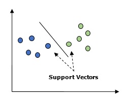
In the above diagram, we have two features. Hence, we first need to plot these two variables in two dimensional space where each point has two co-ordinates, called support vectors. The line splits the data into two different classified groups. This line would be the classifier.

在上图中，我们有两个功能。因此，我们首先需要在二维空间中绘制这两个变量，其中每个点都有两个坐标，称为支持向量。该行将数据分为两个不同的分类组。这行将是分类器。

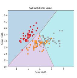
Here, we are going to build an SVM classifier by using scikit-learn and iris dataset. Scikitlearn library has the sklearn.svm module and provides sklearn.svm.svc for classification. The SVM classifier to predict the class of the iris plant based on 4 features are shown below.

在这里，我们将使用scikit-learn和iris数据集来构建SVM分类器。 Scikitlearn库具有sklearn.svm模块，并提供sklearn.svm.svc进行分类。 SVM分类器基于4个特征预测虹膜植物的类别，如下所示。

数据集 (Dataset)

We will use the iris dataset which contains 3 classes of 50 instances each, where each class refers to a type of iris plant. Each instance has the four features namely sepal length, sepal width, petal length and petal width. The SVM classifier to predict the class of the iris plant based on 4 features is shown below.

我们将使用虹膜数据集，该数据集包含3个类别，每个类别有50个实例，其中每个类别都表示一种虹膜植物。每个实例具有四个特征，即萼片长度，萼片宽度，花瓣长度和花瓣宽度。 SVM分类器可基于4个特征预测虹膜植物的分类，如下所示。

核心 (Kernel)

It is a technique used by SVM. Basically these are the functions which take low-dimensional input space and transform it to a higher dimensional space. It converts non-separable problem to separable problem. The kernel function can be any one among linear, polynomial, rbf and sigmoid. In this example, we will use the linear kernel.

这是SVM使用的技术。基本上，这些是占用低维输入空间并将其转换为高维空间的函数。它将不可分离的问题转换为可分离的问题。核函数可以是线性，多项式，rbf和S形中的任何一个。在此示例中，我们将使用线性核。

Let us now import the following packages −

现在让我们导入以下包-


import pandas as pd
import numpy as np
from sklearn import svm, datasets
import matplotlib.pyplot as plt

Now, load the input data −

现在，加载输入数据-


iris = datasets.load_iris()

We are taking first two features −

我们采用了前两个功能-


X = iris.data[:, :2]
y = iris.target

We will plot the support vector machine boundaries with original data. We are creating a mesh to plot.

我们将用原始数据绘制支持向量机的边界。我们正在创建要绘制的网格。


x_min, x_max = X[:, 0].min() - 1, X[:, 0].max() + 1
y_min, y_max = X[:, 1].min() - 1, X[:, 1].max() + 1
h = (x_max / x_min)/100
xx, yy = np.meshgrid(np.arange(x_min, x_max, h),
np.arange(y_min, y_max, h))
X_plot = np.c_[xx.ravel(), yy.ravel()]

We need to give the value of regularization parameter.

我们需要给出正则化参数的值。


C = 1.0

We need to create the SVM classifier object.

我们需要创建SVM分类器对象。


Svc_classifier = svm_classifier.SVC(kernel='linear', 
C=C, decision_function_shape = 'ovr').fit(X, y)
Z = svc_classifier.predict(X_plot)
Z = Z.reshape(xx.shape)
plt.figure(figsize = (15, 5))
plt.subplot(121)
plt.contourf(xx, yy, Z, cmap = plt.cm.tab10, alpha = 0.3)
plt.scatter(X[:, 0], X[:, 1], c = y, cmap = plt.cm.Set1)
plt.xlabel('Sepal length')
plt.ylabel('Sepal width')
plt.xlim(xx.min(), xx.max())
plt.title('SVC with linear kernel')

逻辑回归 (Logistic Regression)

Basically, logistic regression model is one of the members of supervised classification algorithm family. Logistic regression measures the relationship between dependent variables and independent variables by estimating the probabilities using a logistic function.

基本上，逻辑回归模型是监督分类算法家族的成员之一。 Logistic回归通过使用Logistic函数估计概率来测量因变量和自变量之间的关系。

Here, if we talk about dependent and independent variables then dependent variable is the target class variable we are going to predict and on the other side the independent variables are the features we are going to use to predict the target class.

在这里，如果我们谈论因变量和自变量，则因变量是我们要预测的目标类别变量，另一方面，自变量是我们将用来预测目标类别的特征。

In logistic regression, estimating the probabilities means to predict the likelihood occurrence of the event. For example, the shop owner would like to predict the customer who entered into the shop will buy the play station (for example) or not. There would be many features of customer − gender, age, etc. which would be observed by the shop keeper to predict the likelihood occurrence, i.e., buying a play station or not. The logistic function is the sigmoid curve that is used to build the function with various parameters.

在逻辑回归中，估计概率意味着预测事件的可能性发生。例如，商店老板希望预测进入商店的顾客是否会购买游戏台。店主将观察顾客的许多特征-性别，年龄等，以预测可能性的发生，即是否购买游戏机。逻辑函数是S形曲线，用于通过各种参数构建函数。

先决条件 (Prerequisites)

Before building the classifier using logistic regression, we need to install the Tkinter package on our system. It can be installed from https://docs.python.org/2/library/tkinter.html.

在使用逻辑回归构建分类器之前，我们需要在系统上安装Tkinter软件包。可以从https://docs.python.org/2/library/tkinter.html安装。

Now, with the help of the code given below, we can create a classifier using logistic regression −

现在，借助下面给出的代码，我们可以使用逻辑回归创建分类器-

First, we will import some packages −

首先，我们将导入一些包-


import numpy as np
from sklearn import linear_model
import matplotlib.pyplot as plt

Now, we need to define the sample data which can be done as follows −

现在，我们需要定义样本数据，可以按照以下步骤进行操作：


X = np.array([[2, 4.8], [2.9, 4.7], [2.5, 5], [3.2, 5.5], [6, 5], [7.6, 4],
              [3.2, 0.9], [2.9, 1.9],[2.4, 3.5], [0.5, 3.4], [1, 4], [0.9, 5.9]])
y = np.array([0, 0, 0, 1, 1, 1, 2, 2, 2, 3, 3, 3])

Next, we need to create the logistic regression classifier, which can be done as follows −

接下来，我们需要创建逻辑回归分类器，可以按以下步骤进行操作-


Classifier_LR = linear_model.LogisticRegression(solver = 'liblinear', C = 75)

Last but not the least, we need to train this classifier −

最后但并非最不重要的一点，我们需要训练此分类器-


Classifier_LR.fit(X, y)

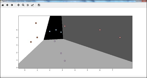
Now, how we can visualize the output? It can be done by creating a function named Logistic_visualize() −

现在，我们如何可视化输出？可以通过创建一个名为Logistic_visualize()的函数来完成-


Def Logistic_visualize(Classifier_LR, X, y):
   min_x, max_x = X[:, 0].min() - 1.0, X[:, 0].max() + 1.0
   min_y, max_y = X[:, 1].min() - 1.0, X[:, 1].max() + 1.0

In the above line, we defined the minimum and maximum values X and Y to be used in mesh grid. In addition, we will define the step size for plotting the mesh grid.

在上一行中，我们定义了在网格网格中使用的最小和最大值X和Y。另外，我们将定义绘制网格的步长。


mesh_step_size = 0.02

Let us define the mesh grid of X and Y values as follows −

让我们定义X和Y值的网格如下：


x_vals, y_vals = np.meshgrid(np.arange(min_x, max_x, mesh_step_size),
                 np.arange(min_y, max_y, mesh_step_size))

With the help of following code, we can run the classifier on the mesh grid −

借助以下代码，我们可以在网格上运行分类器-


output = classifier.predict(np.c_[x_vals.ravel(), y_vals.ravel()])
output = output.reshape(x_vals.shape)
plt.figure()
plt.pcolormesh(x_vals, y_vals, output, cmap = plt.cm.gray)
 
plt.scatter(X[:, 0], X[:, 1], c = y, s = 75, edgecolors = 'black', 
linewidth=1, cmap = plt.cm.Paired)

The following line of code will specify the boundaries of the plot

以下代码行将指定绘图的边界


plt.xlim(x_vals.min(), x_vals.max())
plt.ylim(y_vals.min(), y_vals.max())
plt.xticks((np.arange(int(X[:, 0].min() - 1), int(X[:, 0].max() + 1), 1.0)))
plt.yticks((np.arange(int(X[:, 1].min() - 1), int(X[:, 1].max() + 1), 1.0)))
plt.show()

Now, after running the code we will get the following output, logistic regression classifier −

现在，在运行代码之后，我们将获得以下输出，逻辑回归分类器-

决策树分类器 (Decision Tree Classifier)

A decision tree is basically a binary tree flowchart where each node splits a group of observations according to some feature variable.

决策树基本上是一个二叉树流程图，其中每个节点根据某个特征变量拆分一组观察值。

Here, we are building a Decision Tree classifier for predicting male or female. We will take a very small data set having 19 samples. These samples would consist of two features – ‘height’ and ‘length of hair’.

在这里，我们正在构建用于预测男性或女性的决策树分类器。我们将采用一个非常小的数据集，其中包含19个样本。这些样本将包含两个特征–“高度”和“头发长度”。

先决条件 (Prerequisite)

For building the following classifier, we need to install pydotplus and graphviz. Basically, graphviz is a tool for drawing graphics using dot files and pydotplus is a module to Graphviz’s Dot language. It can be installed with the package manager or pip.

为了构建以下分类器，我们需要安装pydotplus和graphviz 。基本上，graphviz是使用点文件绘制图形的工具，而pydotplus是Graphviz的Dot语言的模块。它可以与软件包管理器或pip一起安装。

Now, we can build the decision tree classifier with the help of the following Python code −

现在，我们可以借助以下Python代码构建决策树分类器：

To begin with, let us import some important libraries as follows −

首先，让我们导入一些重要的库，如下所示：


import pydotplus
from sklearn import tree
from sklearn.datasets import load_iris
from sklearn.metrics import classification_report
from sklearn import cross_validation
import collections

Now, we need to provide the dataset as follows −

现在，我们需要提供如下数据集：


X = [[165,19],[175,32],[136,35],[174,65],[141,28],[176,15],[131,32],
[166,6],[128,32],[179,10],[136,34],[186,2],[126,25],[176,28],[112,38],
[169,9],[171,36],[116,25],[196,25]]

Y = ['Man','Woman','Woman','Man','Woman','Man','Woman','Man','Woman',
'Man','Woman','Man','Woman','Woman','Woman','Man','Woman','Woman','Man']
data_feature_names = ['height','length of hair']

X_train, X_test, Y_train, Y_test = cross_validation.train_test_split
(X, Y, test_size=0.40, random_state=5)

After providing the dataset, we need to fit the model which can be done as follows −

提供数据集后，我们需要拟合模型，可以按以下步骤完成：


clf = tree.DecisionTreeClassifier()
clf = clf.fit(X,Y)

Prediction can be made with the help of the following Python code −

可以借助以下Python代码进行预测-


prediction = clf.predict([[133,37]])
print(prediction)

We can visualize the decision tree with the help of the following Python code −

我们可以在以下Python代码的帮助下可视化决策树-


dot_data = tree.export_graphviz(clf,feature_names = data_feature_names,
            out_file = None,filled = True,rounded = True)
graph = pydotplus.graph_from_dot_data(dot_data)
colors = ('orange', 'yellow')
edges = collections.defaultdict(list)

for edge in graph.get_edge_list():
edges[edge.get_source()].append(int(edge.get_destination()))

for edge in edges: edges[edge].sort()

for i in range(2):dest = graph.get_node(str(edges[edge][i]))[0]
dest.set_fillcolor(colors[i])
graph.write_png('Decisiontree16.png')

It will give the prediction for the above code as [‘Woman’] and create the following decision tree −

它将给出上述代码的预测为['Woman']并创建以下决策树-

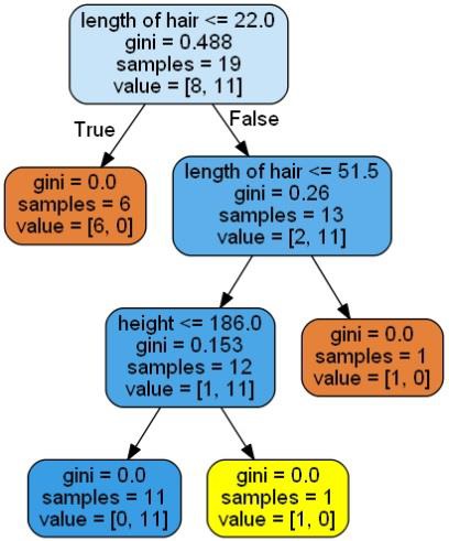
We can change the values of features in prediction to test it.

我们可以更改预测中的要素值以对其进行测试。

随机森林分类器 (Random Forest Classifier)

As we know that ensemble methods are the methods which combine machine learning models into a more powerful machine learning model. Random Forest, a collection of decision trees, is one of them. It is better than single decision tree because while retaining the predictive powers it can reduce over-fitting by averaging the results. Here, we are going to implement the random forest model on scikit learn cancer dataset.

众所周知，集成方法是将机器学习模型组合成更强大的机器学习模型的方法。决策树的集合“随机森林”就是其中之一。它比单一决策树更好，因为在保留预测能力的同时，它可以通过平均结果来减少过度拟合。在这里，我们将在scikit学习癌症数据集上实施随机森林模型。

Import the necessary packages −

导入必要的软件包-


from sklearn.ensemble import RandomForestClassifier
from sklearn.model_selection import train_test_split
from sklearn.datasets import load_breast_cancer
cancer = load_breast_cancer()
import matplotlib.pyplot as plt
import numpy as np

Now, we need to provide the dataset which can be done as follows &minus

现在，我们需要提供可以按以下步骤操作的数据集-


cancer = load_breast_cancer()
X_train, X_test, y_train,
y_test = train_test_split(cancer.data, cancer.target, random_state = 0)

After providing the dataset, we need to fit the model which can be done as follows −

提供数据集后，我们需要拟合模型，可以按以下步骤完成：


forest = RandomForestClassifier(n_estimators = 50, random_state = 0)
forest.fit(X_train,y_train)

Now, get the accuracy on training as well as testing subset: if we will increase the number of estimators then, the accuracy of testing subset would also be increased.

现在，获得训练以及测试子集的准确性：如果我们要增加估计量，那么，测试子集的准确性也将提高。


print('Accuracy on the training subset:(:.3f)',format(forest.score(X_train,y_train)))
print('Accuracy on the training subset:(:.3f)',format(forest.score(X_test,y_test)))

输出量 (Output)


Accuracy on the training subset:(:.3f) 1.0
Accuracy on the training subset:(:.3f) 0.965034965034965

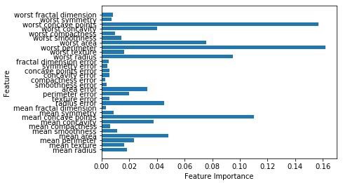
Now, like the decision tree, random forest has the feature_importance module which will provide a better view of feature weight than decision tree. It can be plot and visualize as follows −

现在，像决策树一样，随机森林具有feature_importance模块，该模块将比决策树提供更好的特征权重视图。它可以如下绘制和可视化-


n_features = cancer.data.shape[1]
plt.barh(range(n_features),forest.feature_importances_, align='center')
plt.yticks(np.arange(n_features),cancer.feature_names)
plt.xlabel('Feature Importance')
plt.ylabel('Feature')
plt.show()

分类器的性能 (Performance of a classifier)

After implementing a machine learning algorithm, we need to find out how effective the model is. The criteria for measuring the effectiveness may be based upon datasets and metric. For evaluating different machine learning algorithms, we can use different performance metrics. For example, suppose if a classifier is used to distinguish between images of different objects, we can use the classification performance metrics such as average accuracy, AUC, etc. In one or other sense, the metric we choose to evaluate our machine learning model is very important because the choice of metrics influences how the performance of a machine learning algorithm is measured and compared. Following are some of the metrics −

实施机器学习算法后，我们需要找出模型的有效性。评估有效性的标准可以基于数据集和度量。为了评估不同的机器学习算法，我们可以使用不同的性能指标。例如，假设如果使用分类器来区分不同对象的图像，则我们可以使用分类性能指标，例如平均准确度，AUC等。从某种意义上说，我们选择用来评估机器学习模型的指标是这一点非常重要，因为指标的选择会影响机器学习算法的性能测量和比较方式。以下是一些指标-

混淆矩阵 (Confusion Matrix)

Basically it is used for classification problem where the output can be of two or more types of classes. It is the easiest way to measure the performance of a classifier. A confusion matrix is basically a table with two dimensions namely “Actual” and “Predicted”. Both the dimensions have “True Positives (TP)”, “True Negatives (TN)”, “False Positives (FP)”, “False Negatives (FN)”.

基本上，它用于分类问题，其中输出可以是两种或多种类型的类。这是衡量分类器性能的最简单方法。混淆矩阵基本上是一个具有两个维度的表，即“实际”和“预测”。这两个维度均具有“真阳性(TP)”，“真阴性(TN)”，“假阳性(FP)”，“假阴性(FN)”。

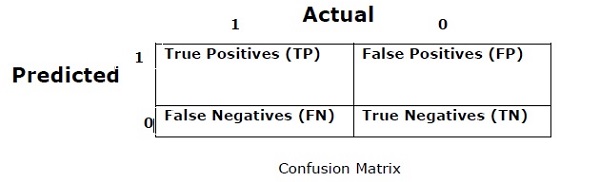
In the confusion matrix above, 1 is for positive class and 0 is for negative class.

在上面的混淆矩阵中，1表示肯定类别，0表示否定类别。

Following are the terms associated with Confusion matrix −

以下是与混淆矩阵相关的术语-

True Positives − TPs are the cases when the actual class of data point was 1 and the predicted is also 1.
真实正值 -TP是数据点的实际类别为1而预测的也是1时的情况。
True Negatives − TNs are the cases when the actual class of the data point was 0 and the predicted is also 0.
真否定 -TN是数据点的实际类别为0而预测也是0时的情况。
False Positives − FPs are the cases when the actual class of data point was 0 and the predicted is also 1.
误报 -FP是指数据点的实际类别为0而预测值为1的情况。
False Negatives − FNs are the cases when the actual class of the data point was 1 and the predicted is also 0.
假阴性 -FN是指数据点的实际类别为1而预测值也为0的情况。

准确性 (Accuracy)

The confusion matrix itself is not a performance measure as such but almost all the performance matrices are based on the confusion matrix. One of them is accuracy. In classification problems, it may be defined as the number of correct predictions made by the model over all kinds of predictions made. The formula for calculating the accuracy is as follows −

混淆矩阵本身并不是性能指标，但是几乎所有性能矩阵都基于混淆矩阵。其中之一是准确性。在分类问题中，可以将其定义为模型在做出的各种预测中做出的正确预测的数量。计算精度的公式如下-

$$Accuracy = \frac{TP+TN}{TP+FP+FN+TN}$$

$$精度= \ frac {TP + TN} {TP + FP + FN + TN} $$

精确 (Precision)

It is mostly used in document retrievals. It may be defined as how many of the returned documents are correct. Following is the formula for calculating the precision −

它主要用于文档检索。它可以定义为多少个返回的文档是正确的。以下是计算精度的公式-

$$Precision = \frac{TP}{TP+FP}$$

$$ Precision = \ frac {TP} {TP + FP} $$

召回或敏感性 (Recall or Sensitivity)

It may be defined as how many of the positives do the model return. Following is the formula for calculating the recall/sensitivity of the model −

可以定义为模型返回多少个肯定值。以下是计算模型的召回率/敏感性的公式-

$$Recall = \frac{TP}{TP+FN}$$

$$ Recall = \ frac {TP} {TP + FN} $$

特异性 (Specificity)

It may be defined as how many of the negatives do the model return. It is exactly opposite to recall. Following is the formula for calculating the specificity of the model −

可以定义为模型返回多少个负数。这与召回完全相反。以下是计算模型特异性的公式-

$$Specificity = \frac{TN}{TN+FP}$$

$$ Specificity = \ frac {TN} {TN + FP} $$

班级失衡问题 (Class Imbalance Problem)

Class imbalance is the scenario where the number of observations belonging to one class is significantly lower than those belonging to the other classes. For example, this problem is prominent in the scenario where we need to identify the rare diseases, fraudulent transactions in bank etc.

类别不平衡是一种情况，其中属于一个类别的观测数量明显少于属于其他类别的观测数量。例如，在需要识别罕见病，银行欺诈交易等情况下，此问题尤为突出。

班级不平衡的例子 (Example of imbalanced classes)

Let us consider an example of fraud detection data set to understand the concept of imbalanced class −

让我们考虑一个欺诈检测数据集的示例，以了解不平衡类的概念-


Total observations = 5000
Fraudulent Observations = 50
Non-Fraudulent Observations = 4950
Event Rate = 1%

解 (Solution)

Balancing the classes’ acts as a solution to imbalanced classes. The main objective of balancing the classes is to either increase the frequency of the minority class or decrease the frequency of the majority class. Following are the approaches to solve the issue of imbalances classes −

平衡班级可以解决班级不平衡的问题。平衡阶级的主要目的是增加少数派的频率或减少多数派的频率。以下是解决不平衡类问题的方法-

重采样 (Re-Sampling)

Re-sampling is a series of methods used to reconstruct the sample data sets − both training sets and testing sets. Re-sampling is done to improve the accuracy of model. Following are some re-sampling techniques −

重采样是用于重建样本数据集(训练集和测试集)的一系列方法。进行重新采样以提高模型的准确性。以下是一些重采样技术-

Random Under-Sampling − This technique aims to balance class distribution by randomly eliminating majority class examples. This is done until the majority and minority class instances are balanced out.
随机欠采样 -此技术旨在通过随机消除多数类别示例来平衡类别分布。这样做直到平衡大多数和少数类实例为止。


Total observations = 5000
Fraudulent Observations = 50
Non-Fraudulent Observations = 4950
Event Rate = 1%

In this case, we are taking 10% samples without replacement from non-fraud instances and then combine them with the fraud instances −

在这种情况下，我们将从非欺诈实例中获取10％的样本而不进行替换，然后将其与欺诈实例合并-

Non-fraudulent observations after random under sampling = 10% of 4950 = 495

随机抽样后的非欺诈性观察= 4950的10％= 495

Total observations after combining them with fraudulent observations = 50+495 = 545

将它们与欺诈性观察合并后的总观察= 50 + 495 = 545

Hence now, the event rate for new dataset after under sampling = 9%

因此，现在，采样后新数据集的事件发生率= 9％

The main advantage of this technique is that it can reduce run time and improve storage. But on the other side, it can discard useful information while reducing the number of training data samples.

该技术的主要优点是可以减少运行时间并改善存储。但另一方面，它可以丢弃有用的信息，同时减少训练数据样本的数量。

Random Over-Sampling − This technique aims to balance class distribution by increasing the number of instances in the minority class by replicating them.
随机过采样 -该技术旨在通过复制少数类来增加实例的数量，从而平衡类的分布。


Total observations = 5000
Fraudulent Observations = 50
Non-Fraudulent Observations = 4950
Event Rate = 1%

In case we are replicating 50 fraudulent observations 30 times then fraudulent observations after replicating the minority class observations would be 1500. And then total observations in the new data after oversampling would be 4950+1500 = 6450. Hence the event rate for the new data set would be 1500/6450 = 23%.

如果我们要复制50次欺诈性观察30次，那么复制少数类观察后的欺诈性观察将为1500次。过采样后新数据中的总观察将为4950 + 1500 =6450。因此，新数据集的事件发生率将是1500/6450 = 23％。

The main advantage of this method is that there would be no loss of useful information. But on the other hand, it has the increased chances of over-fitting because it replicates the minority class events.

这种方法的主要优点是不会丢失有用的信息。但另一方面，由于它复制了少数群体事件，因此出现过度拟合的机会增加。

合奏技巧 (Ensemble Techniques)

This methodology basically is used to modify existing classification algorithms to make them appropriate for imbalanced data sets. In this approach we construct several two stage classifier from the original data and then aggregate their predictions. Random forest classifier is an example of ensemble based classifier.

基本上，此方法用于修改现有分类算法，以使其适合不平衡数据集。在这种方法中，我们从原始数据构造了几个两阶段分类器，然后汇总它们的预测。随机森林分类器是基于集合的分类器的示例。

翻译自: https://www.tutorialspoint.com/artificial_intelligence_with_python/artificial_intelligence_with_python_supervised_learning_classification.htm

cunzai1985

关注

2
点赞
踩
4

收藏

觉得还不错? 一键收藏
0
评论
带有Python的AI –监督学习：分类

带有Python的AI –监督学习：分类 (AI with Python – Supervised Learning: Classification)Advertisements 广告 Previous Page 上一页 Next Page 下一页 In this chapter, we will focus on implementing supervise...
复制链接

扫一扫