autoencoder自编码器原理以及在mnist数据集上的实现

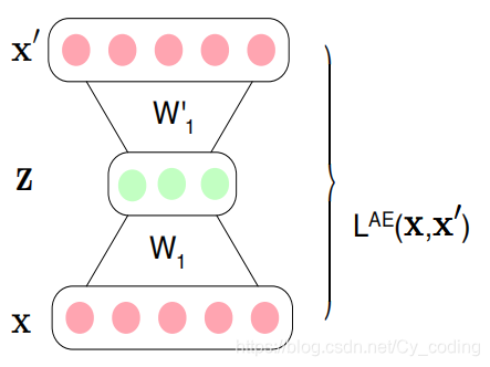
Autoencoder是常见的一种非监督学习的神经网络。它实际由一组相对应的神经网络组成（可以是普通的全连接层，或者是卷积层，亦或者是LSTMRNN等等，取决于项目目的），其目的是将输入数据降维成一个低维度的潜在编码，再通过解码器将数据还原出来。因此autoencoder总是包含了两个部分，编码部分以及解码部分。编码部分负责将输入降维编码，解码部分负责让输出层通过潜在编码还原出输入层。我们的训练目标就是使得输出层与输入层之间的差距最小化。

我们会发现，有一定的风险使得训练出的AE模型是一个恒等函数，这是一个需要尽量避免的问题。

Autoencoder CNN 卷积自编码器

下面我们就用一个简单的基于mnist数据集的实现，来更好地理解autoencoder的原理。
首先是import相关的模块，定义一个用于对比显示输入图像与输出图像的可视化函数。

# Le dataset MNIST
from tensorflow.keras.datasets import mnist
import tensorflow as tf
from tensorflow.keras.layers import Input,Dense, Conv2D, Conv2DTranspose, MaxPooling2D, Flatten, UpSampling2D, Reshape
from tensorflow.keras.models import Model,Sequential
import numpy as np
import matplotlib.pyplot as plt

def MNIST_AE_disp(img_in, img_out, img_idx):

    num_img = len(img_idx)
    plt.figure(figsize=(18, 4))

    for i, image_idx in enumerate(img_idx):
        # 显示输入图像
        ax = plt.subplot(2, num_img, i + 1)
        plt.imshow(img_in[image_idx].reshape(28, 28))
        plt.gray()
        ax.get_xaxis().set_visible(False)
        ax.get_yaxis().set_visible(False)

        # 显示输出图像
        ax = plt.subplot(2, num_img, num_img + i + 1)
        plt.imshow(img_out[image_idx].reshape(28, 28))
        plt.gray()
        ax.get_xaxis().set_visible(False)
        ax.get_yaxis().set_visible(False)
    plt.show()

加载数据并对mnist图像数据进行预处理，包括正则化以及将图片扩充成28，28，1的三维。

(x_train, y_train), (x_test, y_test) = mnist.load_data()
# 正则化 [0, 255] à [0, 1]
x_train=x_train.astype('float32')/float(x_train.