kaggle中的可视化（一）：House Prices

kaggle中预测的get started项目，原文链接。
看原文可以入门特征工程，这里主要说可视化部分，用到matplotlib和seaborn。
导库增加

import seaborn as sns
from scipy.stats import norm
from scipy import stats
from sklearn.preprocessing import StandardScaler

基本信息

获取列名

.cloumns 获取DataFrame的所有列名

df_train.columns

输出

Index(['Id', 'MSSubClass', 'MSZoning', 'LotFrontage', 'LotArea', 'Street',
   'Alley', 'LotShape', 'LandContour', 'Utilities', 'LotConfig',
   'LandSlope', 'Neighborhood', 'Condition1', 'Condition2', 'BldgType',
   'HouseStyle', 'OverallQual', 'OverallCond', 'YearBuilt', 'YearRemodAdd',
   'RoofStyle', 'RoofMatl', 'Exterior1st', 'Exterior2nd', 'MasVnrType',
   'MasVnrArea', 'ExterQual', 'ExterCond', 'Foundation', 'BsmtQual',
   'BsmtCond', 'BsmtExposure', 'BsmtFinType1', 'BsmtFinSF1',
   'BsmtFinType2', 'BsmtFinSF2', 'BsmtUnfSF', 'TotalBsmtSF', 'Heating',
   'HeatingQC', 'CentralAir', 'Electrical', '1stFlrSF', '2ndFlrSF',
   'LowQualFinSF', 'GrLivArea', 'BsmtFullBath', 'BsmtHalfBath', 'FullBath',
   'HalfBath', 'BedroomAbvGr', 'KitchenAbvGr', 'KitchenQual',
   'TotRmsAbvGrd', 'Functional', 'Fireplaces', 'FireplaceQu', 'GarageType',
   'GarageYrBlt', 'GarageFinish', 'GarageCars', 'GarageArea', 'GarageQual',
   'GarageCond', 'PavedDrive', 'WoodDeckSF', 'OpenPorchSF',
   'EnclosedPorch', '3SsnPorch', 'ScreenPorch', 'PoolArea', 'PoolQC',
   'Fence', 'MiscFeature', 'MiscVal', 'MoSold', 'YrSold', 'SaleType',
   'SaleCondition', 'SalePrice'],
  dtype='object')

获取列信息

.describe()用于获取DataFrame某列的基本信息

df_train['SalePrice'].describe()

输出

count      1460.000000
mean     180921.195890
std       79442.502883
min       34900.000000
25%      129975.000000
50%      163000.000000
75%      214000.000000
max      755000.000000
Name: SalePrice, dtype: float64

直方图

用seaborn画直方图

sns.displot(df_train['SalePrice'])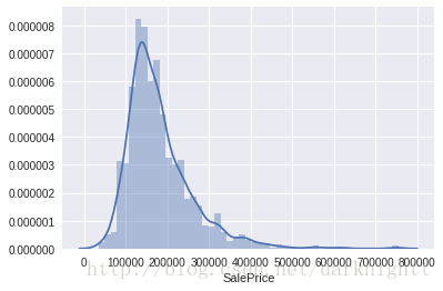

偏度和峰度

.skew() 获取偏度
.kurt() 获取峰度

print("Skewness: %f" % df_train['SalePrice'].skew())
print("Kurtosis: %f" % df_train['SalePrice'].kurt())

输出

Skewness: 1.882876
Kurtosis: 6.536282

散点图

• 以特征GrLivArea为X轴，预测对象SalePrice为Y轴，观察相关性，如是否有线性关系

var = 'GrLivArea'
data = pd.concat([df_train['SalePrice'], df_train[var]], axis=1)
data.plot.scatter(x=var, y='SalePrice', ylim=(0,800000));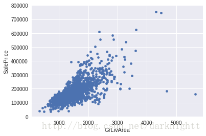

• 用seaborn的.pairplot() 画很多散点图

sns.set()
cols = ['SalePrice', 'OverallQual', 'GrLivArea', 'GarageCars', 'TotalBsmtSF', 'FullBath', 'YearBuilt']
sns.pairplot(df_train[cols], size = 2.5)
plt.show();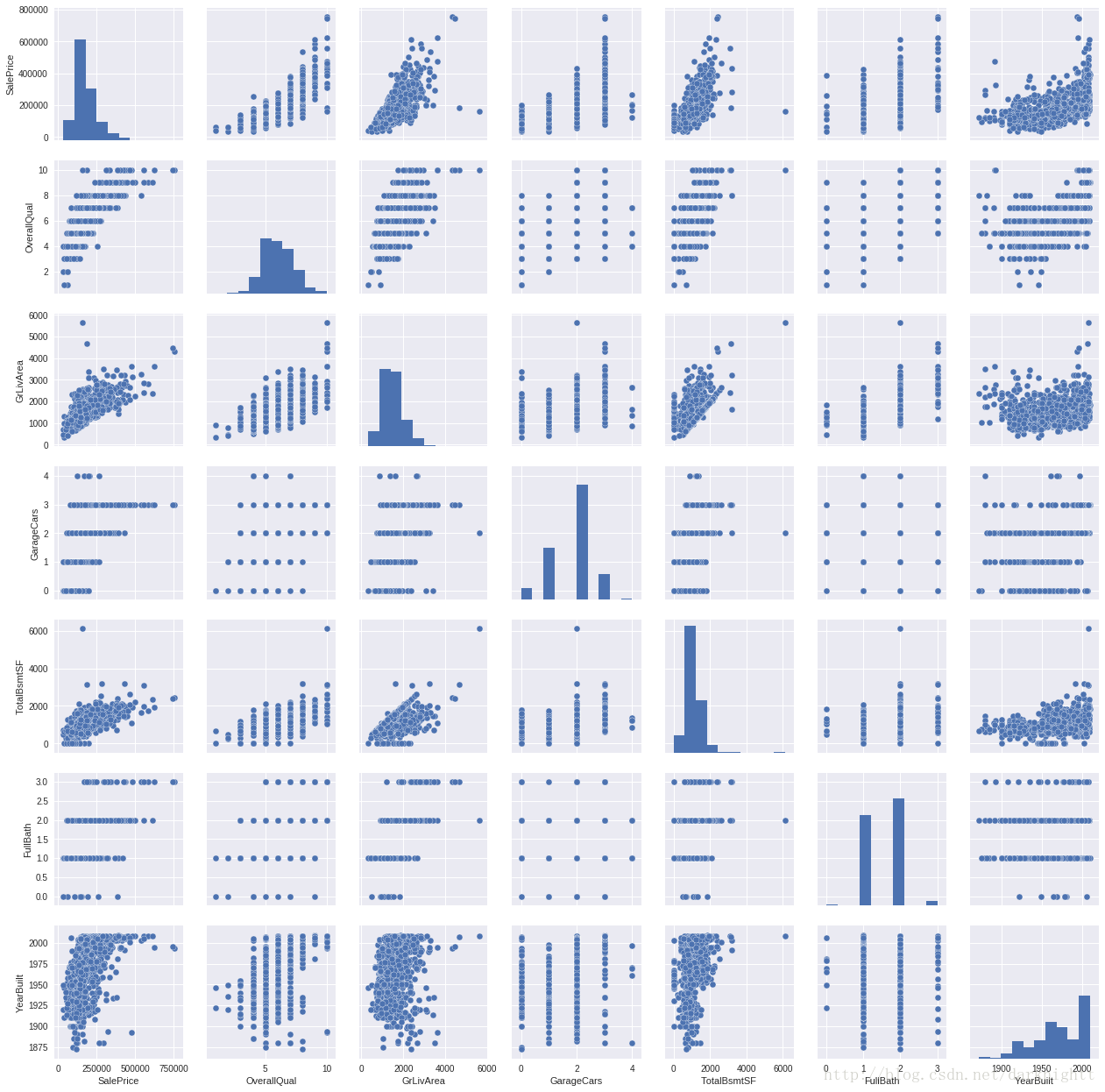

盒图

用seaborn的.boxplot() 方法画盒图，观察特征OverallQual与SalePrice的关系

var = 'OverallQual'
data = pd.concat([df_train['SalePrice'], df_train[var]], axis=1)
f, ax = plt.subplots(figsize=(8, 6))
fig = sns.boxplot(x=var, y="SalePrice", data=data)
fig.axis(ymin=0, ymax=800000);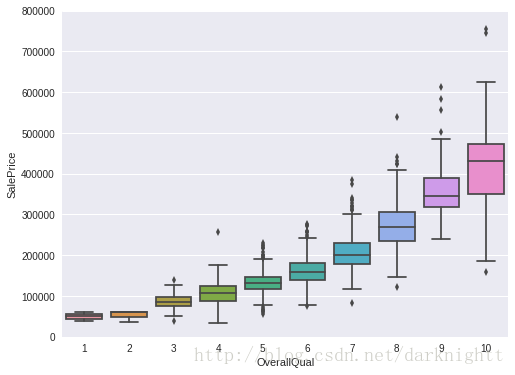

热图

seaborn库的.heatmap() 方法
协方差矩阵热图，颜色越深代表相关性越强

corrmat = df_train.corr()
f, ax = plt.subplots(figsize=(12, 9))
sns.heatmap(corrmat, vmax=.8, square=True);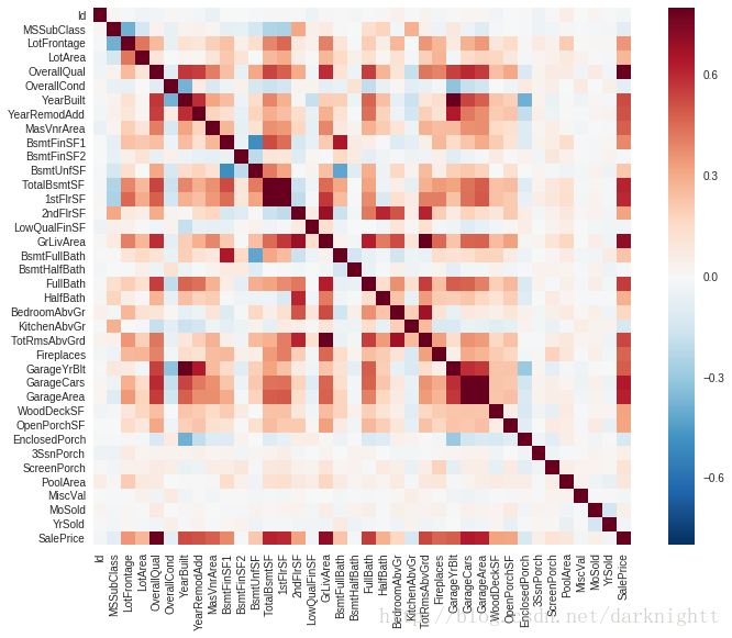

选取与SalePrice相关系数最高的10个特征作热图，显示相关系数

k = 10 #number of variables for heatmap
cols = corrmat.nlargest(k, 'SalePrice')['SalePrice'].index
cm = np.corrcoef(df_train[cols].values.T)
sns.set(font_scale=1.25)
hm = sns.heatmap(cm, cbar=True, annot=True, square=True, fmt='.2f', annot_kws={'size': 10}, yticklabels=cols.values, xticklabels=cols.values)
plt.show()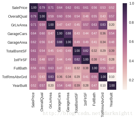

缺失值

计算各特征对应缺失值占比，返回前20的情况

total = df_train.isnull().sum().sort_values(ascending=False)
percent = (df_train.isnull().sum()/df_train.isnull().count()).sort_values(ascending=False)
missing_data = pd.concat([total, percent], axis=1, keys=['Total', 'Percent'])
missing_data.head(20)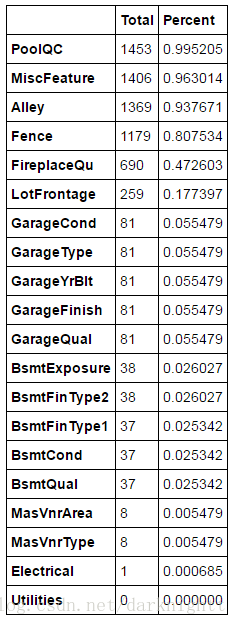

离群点

单变量分析

首先用标准化（标准化不会改变数据相对分布的特性）把数据转变成正态分布，分别查看最大和最小的十个值

saleprice_scaled = StandardScaler().fit_transform(df_train['SalePrice'][:,np.newaxis]);
low_range = saleprice_scaled[saleprice_scaled[:,0].argsort()][:10]
high_range= saleprice_scaled[saleprice_scaled[:,0].argsort()][-10:]
print('outer range (low) of the distribution:')
print(low_range)
print('\nouter range (high) of the distribution:')
print(high_range)

输出

outer range (low) of the distribution:
[[-1.83820775]
 [-1.83303414]
 [-1.80044422]
 [-1.78282123]
 [-1.77400974]
 [-1.62295562]
 [-1.6166617 ]
 [-1.58519209]
 [-1.58519209]
 [-1.57269236]]

outer range (high) of the distribution:
[[ 3.82758058]
 [ 4.0395221 ]
 [ 4.49473628]
 [ 4.70872962]
 [ 4.728631  ]
 [ 5.06034585]
 [ 5.42191907]
 [ 5.58987866]
 [ 7.10041987]
 [ 7.22629831]]

可以发现，Low range值偏离原点并且都比较相近，High range离远点较远，7.很可能是异常值

双变量分析

以GrLivArea为X轴，SalePrice为y轴画散点图

var = 'GrLivArea'
data = pd.concat([df_train['SalePrice'], df_train[var]], axis=1)
data.plot.scatter(x=var, y='SalePrice', ylim=(0,800000));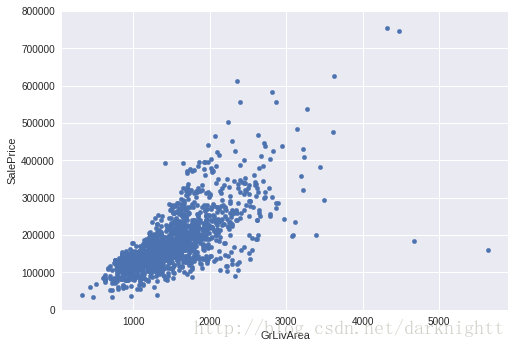

从图中看出二者很可能有线性关系，则图中右下方的两个点作为异常值舍弃

df_train.sort_values(by = 'GrLivArea', ascending = False)[:2]
df_train = df_train.drop(df_train[df_train['Id'] == 1299].index)
df_train = df_train.drop(df_train[df_train['Id'] == 524].index)

正态化

scipy库中stats对象的.probplot() 方法拟合一个高斯正态分布，以SalePrice为例

sns.distplot(df_train['SalePrice'], fit=norm);
fig = plt.figure()
res = stats.probplot(df_train['SalePrice'], plot=plt)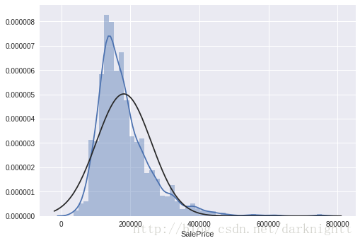

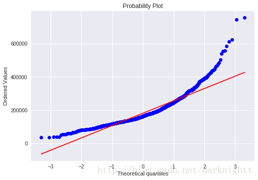
可以看到数据呈正偏态分布，现在我们想把它转变成正太分布。统计学里面一个常用的做法就是对SalePrice的取log。

df_train['SalePrice'] = np.log(df_train['SalePrice'])
sns.distplot(df_train['SalePrice'], fit=norm);
fig = plt.figure()
res = stats.probplot(df_train['SalePrice'], plot=plt)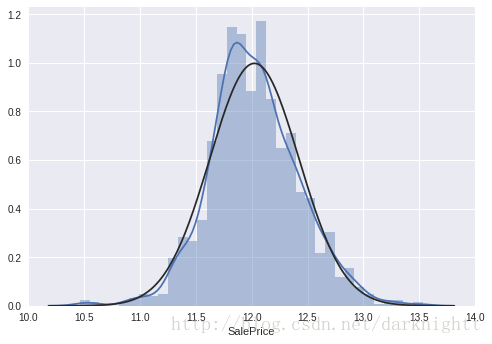

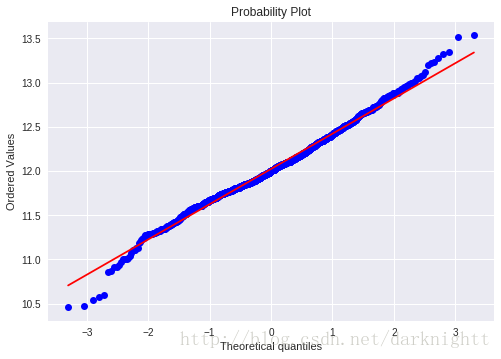
可以看到对SalePrice做了log变换之后近似于正态分布了