


由于篇幅过长,一共分为八个文档,此为第三部分,内容如下目录:
Trigger/Picker Tutorial(触发器/拾取器教程)
Poles and Zeros, Frequency Response(零极点和频率响应)
Seismometer Correction/Simulation(地震仪校准和仿真)
Trigger/Picker Tutorial(触发器/拾取器教程)
教程中所用测试数据在这里trigger_data.zip.下载。
触发器的实现如[Withers1998].中所述。参考[Trnkoczy2012].求取STA / LTA类型触发器的正确触发参数信息。请注意使用obspy中提供的Stream.trigger和Trace.trigger作为便利方法。
使用read()函数读取数据文件到Trace对象。
from obspy.core import read

st = read("https://examples.obspy.org/ev0_6.a01.gse2")

st = st.select(component="Z")

tr = st[0]
数据类型可以被自动检测。这个教程中最重要的是掌握Trace中的各个属性:
Table 7
| tr.data | Numpy.ndarray |
| tr.stats | 包含头信息的类似字典的类 |
| tr.stats.sampling_rate | 采样率 |
| tr.stats.npts | 采样的数量 |
下面的例子展示了数据文件头信息,并绘制了数据图像:
>>>print(tr.stats)

         network:

         station: EV0_6

        location:

         channel: EHZ

       starttime: 1970-01-01T01:00:00.000000Z

         endtime: 1970-01-01T01:00:59.995000Z

   sampling_rate: 200.0

           delta: 0.005

            npts: 12000

           calib: 1.0

         _format: GSE2

            gse2: AttribDict({'instype': '      ', 'datatype': 'CM6', 'hang': 0.0, 'auxid': '    ', 'vang': -1.0, 'calper': 1.0})
使用Trace对象的plot()方法绘制:
>>>tr.plot(type="relative") 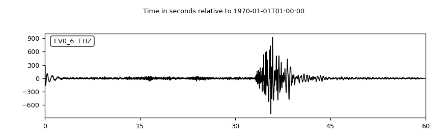
在加载完数据后,我们可以将波形数据传递给obspy.signal.trigger中定义的以下触发器例程:
Table 8
| recursive_sta_lta(a, nsta, nlta) | 递归STA / LTA |
| carl_sta_trig(a, nsta, nlta, ratio, quiet) | 计算carlSTAtrig特征函数 |
| classic_sta_lta(a, nsta, nlta) | 计算标准STA / LTA |
| delayed_sta_lta(a, nsta, nlta) | 延迟的STA / LTA |
| z_detect(a, nsta) | Z检测器 |
| pk_baer(reltrc, samp_int, tdownmax, ...) | P_picker包装 |
| ar_pick(a, b, c, samp_rate, f1, f2, lta_p, ...) | 使用AR-AIC + STA / LTA算法检测P和S的到达 |
每个函数的帮助信息都有HTML格式信息或通常的Python方式查询:
>>>from obspy.signal.trigger import classic_sta_lta

>>>help(classic_sta_lta)
设置触发器主要经由以下两个步骤:1)计算特征函数,2)根据特征函数的值设置picks
所有的例子中,读取数据加载模型的命令如下:
>>>from obspy.core import read

>>>from obspy.signal.trigger import plot_trigger

>>>trace= read("https://examples.obspy.org/ev0_6.a01.gse2")[0]

>>>df = trace.stats.sampling_rate>>>from obspy.signal.trigger import classic_sta_lta
>>>cft = classic_sta_lta(trace.data, int(5 * df), int(10 * df))
>>>plot_trigger(trace, cft, 1.5, 0.5)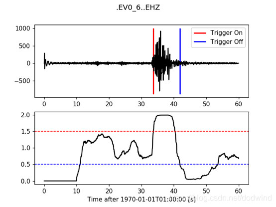
Z探测
>>>from obspy.signal.trigger import z_detect

>>>cft = z_detect(trace.data, int(10 * df))

>>>plot_trigger(trace, cft, -0.4, -0.3)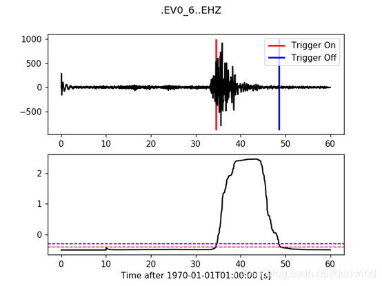
>>>from obspy.signal.trigger import recursive_sta_lta

>>>cft = recursive_sta_lta(trace.data, int(5 * df), int(10 * df))

>>>plot_trigger(trace, cft, 1.2, 0.5)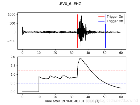
卡尔-STA-触发
>>>from obspy.signal.trigger import carl_sta_trig

>>>cft = carl_sta_trig(trace.data, int(5 * df), int(10 * df), 0.8, 0.8)

>>>plot_trigger(trace, cft, 20.0, -20.0)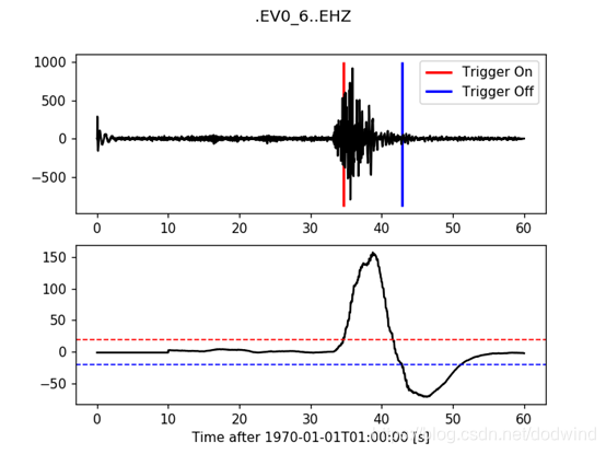
>>>from obspy.signal.trigger import delayed_sta_lta

>>>cft = delayed_sta_lta(trace.data, int(5 * df), int(10 * df))

>>>plot_trigger(trace, cft, 5, 10)
这个例子中展示了一个由4个台站组成的网络联合触发器,每个触发器使用递归STA/LTA。波形数据持续四分钟,包含四个事件。其中两个很容易识别(MI 1-2),剩下的两个(MI <= 0)需要调整好合适的触发器设定才能被检测到.
首先我们将所有波形数据整合于一个Stream对象中,使用的数据能从我们的网络服务器中获取:
>>>from obspy.core import Stream, read

>>>st = Stream()

>>>files = ["BW.UH1..SHZ.D.2010.147.cut.slist.gz",

         "BW.UH2..SHZ.D.2010.147.cut.slist.gz",

         "BW.UH3..SHZ.D.2010.147.cut.slist.gz",

         "BW.UH4..SHZ.D.2010.147.cut.slist.gz"]

>>>for filename in files:

st += read("https://examples.obspy.org/" + filename)
在经过带通滤波之后,对所有数据进行联合tiggering。使用递归STA/LTA,触发器参数设置:时间窗0.5~10秒,开阈值3.5,关阈值1,例子中每个台站的权重相同,联合总阈值为3。对于更复杂的网络,可以为每个台站/信道分配不同的权重。为了保留源数据,我们使用源Stream的副本进行处理:
>>>st.filter('bandpass', freqmin=10, freqmax=20)  # optional prefiltering

>>>from obspy.signal.trigger import coincidence_trigger

>>>st2 = st.copy()

>>>trig = coincidence_trigger("recstalta", 3.5, 1, st2, 3, sta=0.5, lta=10)
使用pprint打印结果显示如下:
>>>from pprint import pprint

>>>pprint(trig)

[{'coincidence_sum': 4.0,

  'duration': 4.5299999713897705,

  'stations': ['UH3', 'UH2', 'UH1', 'UH4'],

  'time': UTCDateTime(2010, 5, 27, 16, 24, 33, 190000),

  'trace_ids': ['BW.UH3..SHZ', 'BW.UH2..SHZ', 'BW.UH1..SHZ',

                'BW.UH4..SHZ']},

 {'coincidence_sum': 3.0,

  'duration': 3.440000057220459,

  'stations': ['UH2', 'UH3', 'UH1'],

  'time': UTCDateTime(2010, 5, 27, 16, 27, 1, 260000),

  'trace_ids': ['BW.UH2..SHZ', 'BW.UH3..SHZ', 'BW.UH1..SHZ']},

 {'coincidence_sum': 4.0,

  'duration': 4.7899999618530273,

  'stations': ['UH3', 'UH2', 'UH1', 'UH4'],

  'time': UTCDateTime(2010, 5, 27, 16, 27, 30, 490000),

  'trace_ids': ['BW.UH3..SHZ', 'BW.UH2..SHZ', 'BW.UH1..SHZ',

                'BW.UH4..SHZ']}]
使用当前这些设定触发器报告了三个事件,提供每个(可能的)事件的开始时间和持续时间。此外还提供台站名和trace ID的列表,其按台站触发时间排序,这可以帮助我们对事件发生的位置有一个初始的粗略的想法。我们可以设定“details = True”来访问更多信息。
>>>st2 = st.copy()

>>>trig = coincidence_trigger("recstalta", 3.5, 1, st2, 3, sta=0.5, lta=10,details=True)
为了显示清晰,我们这里只展示了结果中的第一项:
>>>pprint(trig[0])

{'cft_peak_wmean': 19.561900329259956,

 'cft_peaks': [19.535644192544272,

               19.872432918501264,

               19.622171410201297,

               19.217352795792998],

 'cft_std_wmean': 5.4565629691954713,

 'cft_stds': [5.292458320417178,

              5.6565387957966404,

              5.7582248973698507,

              5.1190298631982163],

 'coincidence_sum': 4.0,

 'duration': 4.5299999713897705,

 'stations': ['UH3', 'UH2', 'UH1', 'UH4'],

 'time': UTCDateTime(2010, 5, 27, 16, 24, 33, 190000),

 'trace_ids': ['BW.UH3..SHZ', 'BW.UH2..SHZ', 'BW.UH1..SHZ', 'BW.UH4..SHZ']}
在此,提供了关于单个台站触发器的特征函数的峰值和标准偏差等一些附加信息。此外也计算有二者的加权平均值。这些值可以帮助我们区分某些有问题的网络触发器。
这个例子是普通网络联合触发器的扩展。已知事件的波形可以被用于检测单个台站触发器的波形的相似性。如果相似度超过了相应的相似性阈值,即使联合值不及设定的最小值,该事件触发也会被记录到结果列表。使用这种方法,可以在某个台站有非常相似的波形记录时完成探测即使其他台站由于某些原因未能探测到触发(例如台站临时停电或者噪声水平高等因素)。可以为任何台站提供随意数量的波形模板。由于必要的交叉相关计算时间会显著增加。在该例中我们使用两个三成分组合事件模板应用于公共网络触发器的垂直向。
>>>from obspy.core import Stream, read, UTCDateTime

>>>st = Stream()

>>>files = ["BW.UH1..SHZ.D.2010.147.cut.slist.gz",

         "BW.UH2..SHZ.D.2010.147.cut.slist.gz",

         "BW.UH3..SHZ.D.2010.147.cut.slist.gz",

         "BW.UH3..SHN.D.2010.147.cut.slist.gz",

         "BW.UH3..SHE.D.2010.147.cut.slist.gz",

         "BW.UH4..SHZ.D.2010.147.cut.slist.gz"]

>>>for filename in files:

    st += read("https://examples.obspy.org/" + filename)

>>>st.filter('bandpass', freqmin=10, freqmax=20)  # optional prefiltering
这里我们为单个台站设置一个事件模板的字典。指定时间为P波的精确到时,事件持续时间(包括S波)约2.5秒。在UH3台站我们使用两个三分量事件模板数据,在UH1台站我们仅使用一个事件模板的垂直向数据。
>>>times = ["2010-05-27T16:24:33.095000", "2010-05-27T16:27:30.370000"]

>>>event_templates = {"UH3": []}

>>>for t in times:

    t = UTCDateTime(t)

    st_ = st.select(station="UH3").slice(t, t + 2.5)

    event_templates["UH3"].append(st_)

>>>t = UTCDateTime("2010-05-27T16:27:30.574999")

>>>st_ = st.select(station="UH1").slice(t, t + 2.5)

>>>event_templates["UH1"] = [st_]
下一步提供事件模板波形和相似度阈值。注意重合总和设置是4,我们手动设定只使用相同站点重合值为1的垂直分量。
>>>from obspy.signal.trigger import coincidence_trigger

>>>st2 = st.copy()

>>>trace_ids = {"BW.UH1..SHZ": 1,

             "BW.UH2..SHZ": 1,

             "BW.UH3..SHZ": 1,

             "BW.UH4..SHZ": 1}

>>>similarity_thresholds = {"UH1": 0.8, "UH3": 0.7}

>>>trig = coincidence_trigger("classicstalta", 5, 1, st2, 4, sta=0.5,

                          lta=10, trace_ids=trace_ids,

                          event_templates=event_templates,

                          similarity_threshold=similarity_thresholds)
现在的结果包含两个事件触发,其并不超过设置的最小重合阈值但是和至少一个事件模板的相似度超过设定阈值。在检查事件触发器时,请注意1.0的值,我们为此示例提取了事件模板。
>>>from pprint import pprint

>>>pprint(trig)

[{'coincidence_sum': 4.0,

  'duration': 4.1100001335144043,

  'similarity': {'UH1': 0.9414944738498271, 'UH3': 1.0},

  'stations': ['UH3', 'UH2', 'UH1', 'UH4'],

  'time': UTCDateTime(2010, 5, 27, 16, 24, 33, 210000),

  'trace_ids': ['BW.UH3..SHZ', 'BW.UH2..SHZ', 'BW.UH1..SHZ', 'BW.UH4..SHZ']},

 {'coincidence_sum': 3.0,

  'duration': 1.9900000095367432,

  'similarity': {'UH1': 0.65228204570577764, 'UH3': 0.72679293429214198},

  'stations': ['UH3', 'UH1', 'UH2'],

  'time': UTCDateTime(2010, 5, 27, 16, 25, 26, 710000),

  'trace_ids': ['BW.UH3..SHZ', 'BW.UH1..SHZ', 'BW.UH2..SHZ']},

 {'coincidence_sum': 3.0,

  'duration': 1.9200000762939453,

  'similarity': {'UH1': 0.89404458774338103, 'UH3': 0.74581409371425222},

  'stations': ['UH2', 'UH1', 'UH3'],

  'time': UTCDateTime(2010, 5, 27, 16, 27, 2, 260000),

  'trace_ids': ['BW.UH2..SHZ', 'BW.UH1..SHZ', 'BW.UH3..SHZ']},

 {'coincidence_sum': 4.0,

  'duration': 4.0299999713897705,

  'similarity': {'UH1': 1.0, 'UH3': 1.0},

  'stations': ['UH3', 'UH2', 'UH1', 'UH4'],

  'time': UTCDateTime(2010, 5, 27, 16, 27, 30, 510000),

  'trace_ids': ['BW.UH3..SHZ', 'BW.UH2..SHZ', 'BW.UH1..SHZ', 'BW.UH4..SHZ']}]
对于pk_bear(),输入单位秒,输出为样本。
>>>from obspy.core import read

>>>from obspy.signal.trigger import pk_baer

>>>trace = read("https://examples.obspy.org/ev0_6.a01.gse2")[0]

>>>df = trace.stats.sampling_rate

>>>p_pick, phase_info = pk_baer(trace.data, df,

                            20, 60, 7.0, 12.0, 100, 100)

>>>print(p_pick)

6894

>>print(phase_info)

EPU3

>>>print(p_pick / df)

34.47
生成值34.47 EPU3含义是P波选择34.47s相位信息EPU3。
对于ar_pick(),输入和输出单位都是秒。
>>>from obspy.core import read

>>>from obspy.signal.trigger import ar_pick

>>>tr1 = read('https://examples.obspy.org/loc_RJOB20050801145719850.z.gse2')[0]

>>>tr2 = read('https://examples.obspy.org/loc_RJOB20050801145719850.n.gse2')[0]

>>>tr3 = read('https://examples.obspy.org/loc_RJOB20050801145719850.e.gse2')[0]

>>>df = tr1.stats.sampling_rate

>>>p_pick, s_pick = ar_pick(tr1.data, tr2.data, tr3.data, df,

                         1.0, 20.0, 1.0, 0.1, 4.0, 1.0, 2, 8, 0.1, 0.2)

>>>print(p_pick)

30.6350002289

>>>print(s_pick)

31.2800006866
输出的30.6350002289和31.2800006866意思是在30.64s的P波和在31.28s的S波被拾取出来。
这是一个更复杂的例子,数据通过ArcLink检索,结果被一步一步的绘制,代码如下:
import matplotlib.pyplot as plt


import obspy

from obspy.clients.arclink import Client

from obspy.signal.trigger import recursive_sta_lta, trigger_onset


# Retrieve waveforms via ArcLink

client = Client(host="erde.geophysik.uni-muenchen.de", port=18001,

                user="test@obspy.de")

t = obspy.UTCDateTime("2009-08-24 00:19:45")

st = client.get_waveforms('BW', 'RTSH', '', 'EHZ', t, t + 50)


# For convenience

tr = st[0]  # only one trace in mseed volume

df = tr.stats.sampling_rate


# Characteristic function and trigger onsets

cft = recursive_sta_lta(tr.data, int(2.5 * df), int(10. * df))

on_of = trigger_onset(cft, 3.5, 0.5)


# Plotting the results

ax = plt.subplot(211)

plt.plot(tr.data, 'k')

ymin, ymax = ax.get_ylim()

plt.vlines(on_of[:, 0], ymin, ymax, color='r', linewidth=2)

plt.vlines(on_of[:, 1], ymin, ymax, color='b', linewidth=2)

plt.subplot(212, sharex=ax)

plt.plot(cft, 'k')

plt.hlines([3.5, 0.5], 0, len(cft), color=['r', 'b'], linestyle='--')

plt.axis('tight')

plt.show()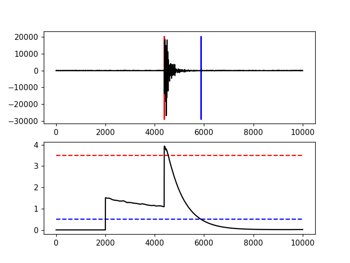
Poles and Zeros, Frequency Response(零极点和频率响应)
注意:使用read_inventory()读取元信息到Inventory对象(和相关的Network、Station、Channel、Response子对象)中。参考Inventory.plot_response() or Response.plot()使用便捷的方法绘制波德图。
下面的代码展示了如何计算并显示LE-3D/1S地震仪的频率响应,其采样间隔0.005s,傅里叶快速变换16384个点。我们希望相位角从0到2π,而不是从-π到π的输出。
import numpy as np

import matplotlib.pyplot as plt


from obspy.signal.invsim import paz_to_freq_resp


poles = [-4.440 + 4.440j, -4.440 - 4.440j, -1.083 + 0.0j]

zeros = [0.0 + 0.0j, 0.0 + 0.0j, 0.0 + 0.0j]

scale_fac = 0.4


h, f = paz_to_freq_resp(poles, zeros, scale_fac, 0.005, 16384, freq=True)


plt.figure()

plt.subplot(121)

plt.loglog(f, abs(h))

plt.xlabel('Frequency [Hz]')

plt.ylabel('Amplitude')


plt.subplot(122)

phase = 2 * np.pi + np.unwrap(np.angle(h))

plt.semilogx(f, phase)

plt.xlabel('Frequency [Hz]')

plt.ylabel('Phase [radian]')

# ticks and tick labels at multiples of pi

plt.yticks(

    [0, np.pi / 2, np.pi, 3 * np.pi / 2, 2 * np.pi],

    ['$0$', r'$\frac{\pi}{2}$', r'$\pi$', r'$\frac{3\pi}{2}$', r'$2\pi$'])

plt.ylim(-0.2, 2 * np.pi + 0.2)

# title, centered above both subplots

plt.suptitle('Frequency Response of LE-3D/1s Seismometer')

# make more room in between subplots for the ylabel of right plot

plt.subplots_adjust(wspace=0.3)

plt.show()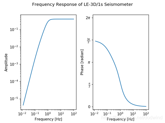
Seismometer Correction/Simulation(地震仪校准和仿真)
使用StationXML文件或者常用的Inventory对象
当使用FDSN client时,响应可以被直接附加在波形上,后续的删除可以使用Stream.remove_response():
from obspy import UTCDateTime

from obspy.clients.fdsn import Client


t1 = UTCDateTime("2010-09-3T16:30:00.000")

t2 = UTCDateTime("2010-09-3T17:00:00.000")

fdsn_client = Client('IRIS')

# Fetch waveform from IRIS FDSN web service into a ObsPy stream object

# and automatically attach correct response

st = fdsn_client.get_waveforms(network='NZ', station='BFZ', location='10',

                               channel='HHZ', starttime=t1, endtime=t2,

                               attach_response=True)

# define a filter band to prevent amplifying noise during the deconvolution

pre_filt = (0.005, 0.006, 30.0, 35.0)

st.remove_response(output='DISP', pre_filt=pre_filt)
该方法同样适用于Inventory对象:
from obspy import read, read_inventory


# simply use the included example waveform

st = read()

# the corresponding response is included in ObsPy as a StationXML file

inv = read_inventory()

# the routine automatically picks the correct response for each trace

# define a filter band to prevent amplifying noise during the deconvolution

pre_filt = (0.005, 0.006, 30.0, 35.0)

st.remove_response(inventory=inv, output='DISP', pre_filt=pre_filt)
使用绘图选项,可以在频域中显示响应消除期间的各个步骤,用以检查pre_filt和water_level选项,以稳定倒置仪器响应谱的反卷积。
from obspy import read, read_inventory


st = read("/path/to/IU_ULN_00_LH1_2015-07-18T02.mseed")

tr = st[0]

inv = read_inventory("/path/to/IU_ULN_00_LH1.xml")

pre_filt = [0.001, 0.005, 10, 20]

tr.remove_response(inventory=inv, pre_filt=pre_filt, output="DISP",

                   water_level=60, plot=True)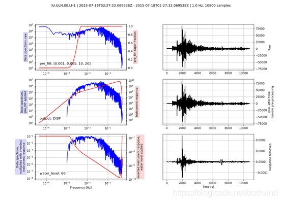
使用RESP文件
使用RESP文件计算仪器响应信息。
import matplotlib.pyplot as plt


import obspy

from obspy.core.util import NamedTemporaryFile

from obspy.clients.fdsn import Client as FDSN_Client

from obspy.clients.iris import Client as OldIris_Client


# MW 7.1 Darfield earthquake, New Zealand

t1 = obspy.UTCDateTime("2010-09-3T16:30:00.000")

t2 = obspy.UTCDateTime("2010-09-3T17:00:00.000")


# Fetch waveform from IRIS FDSN web service into a ObsPy stream object

fdsn_client = FDSN_Client("IRIS")

st = fdsn_client.get_waveforms('NZ', 'BFZ', '10', 'HHZ', t1, t2)


# Download and save instrument response file into a temporary file

with NamedTemporaryFile() as tf:

    respf = tf.name

    old_iris_client = OldIris_Client()

    # fetch RESP information from "old" IRIS web service, see obspy.fdsn

    # for accessing the new IRIS FDSN web services

    old_iris_client.resp('NZ', 'BFZ', '10', 'HHZ', t1, t2, filename=respf)


    # make a copy to keep our original data

    st_orig = st.copy()


    # define a filter band to prevent amplifying noise during the deconvolution

    pre_filt = (0.005, 0.006, 30.0, 35.0)


    # this can be the date of your raw data or any date for which the

    # SEED RESP-file is valid

    date = t1


    seedresp = {'filename': respf,  # RESP filename

                # when using Trace/Stream.simulate() the "date" parameter can

                # also be omitted, and the starttime of the trace is then used.

                'date': date,

                # Units to return response in ('DIS', 'VEL' or ACC)

                'units': 'DIS'

                }


    # Remove instrument response using the information from the given RESP file

    st.simulate(paz_remove=None, pre_filt=pre_filt, seedresp=seedresp)


# plot original and simulated data

tr = st[0]

tr_orig = st_orig[0]

time = tr.times()


plt.subplot(211)

plt.plot(time, tr_orig.data, 'k')

plt.ylabel('STS-2 [counts]')

plt.subplot(212)

plt.plot(time, tr.data, 'k')

plt.ylabel('Displacement [m]')

plt.xlabel('Time [s]')

plt.show()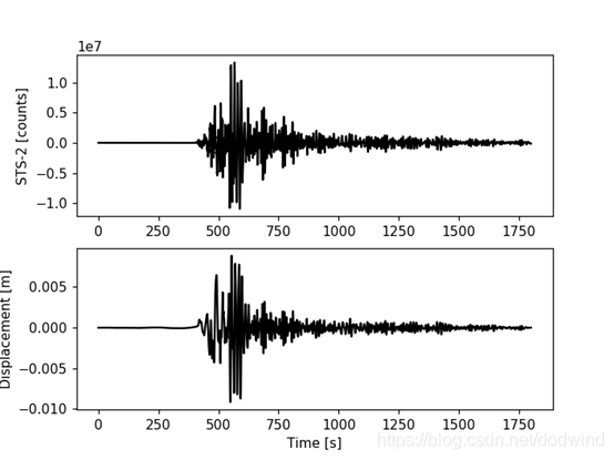
使用缺/全数据SEED文件(或XMLSEED文件)
使用无数据SEED文件创建的Parser对象也可以被使用。然后对于每条轨迹提取RESP响应数据。当使用Stream或Trace中的simulate()便捷方法时,“data”参数可以省略。
import obspy

from obspy.io.xseed import Parser


st = obspy.read("https://examples.obspy.org/BW.BGLD..EH.D.2010.037")

parser = Parser("https://examples.obspy.org/dataless.seed.BW_BGLD")

st.simulate(seedresp={'filename': parser, 'units': "DIS"})使用PAZ字典
下面的脚本展示了如何使用给定的零极点模拟1Hz的STS-2地震仪。零极点、增益(归一化因子A0)、灵敏度(总灵敏度)被指定为字典的关键字。
import obspy

from obspy.signal.invsim import corn_freq_2_paz


paz_sts2 = {

    'poles': [-0.037004 + 0.037016j, -0.037004 - 0.037016j, -251.33 + 0j,

              - 131.04 - 467.29j, -131.04 + 467.29j],

    'zeros': [0j, 0j],

    'gain': 60077000.0,

    'sensitivity': 2516778400.0}

paz_1hz = corn_freq_2_paz(1.0, damp=0.707)  # 1Hz instrument

paz_1hz['sensitivity'] = 1.0


st = obspy.read()

# make a copy to keep our original data

st_orig = st.copy()


# Simulate instrument given poles, zeros and gain of

# the original and desired instrument

st.simulate(paz_remove=paz_sts2, paz_simulate=paz_1hz)


# plot original and simulated data

st_orig.plot()

st.plot()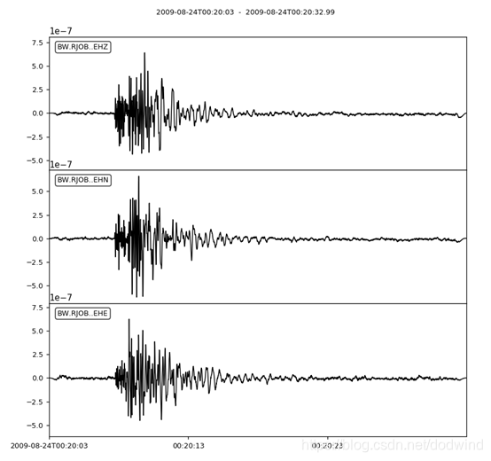
更多自定义的绘图设置可以使用matplotlib手动设定:
import numpy as np

import matplotlib.pyplot as plt


tr = st[0]

tr_orig = st_orig[0]


t = np.arange(tr.stats.npts) / tr.stats.sampling_rate


plt.subplot(211)

plt.plot(t, tr_orig.data, 'k')

plt.ylabel('STS-2 [counts]')

plt.subplot(212)

plt.plot(t, tr.data, 'k')

plt.ylabel('1Hz Instrument [m/s]')

plt.xlabel('Time [s]')

plt.show()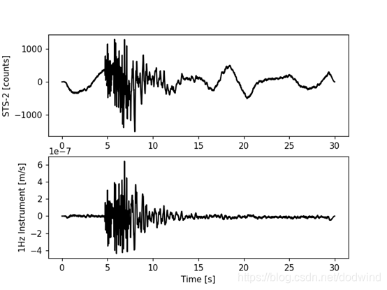


 7521
7521

 被折叠的 条评论
为什么被折叠?
被折叠的 条评论
为什么被折叠?
 到【灌水乐园】发言


